Introduction

One of the most fundamental challenges in science and data analysis is distinguishing correlation from causation. While machine learning models are excellent at finding patterns (correlations), they often struggle to tell us why things happen (causation). To bridge this gap, researchers rely on Directed Acyclic Graphs (DAGs) to map out causal relationships between variables.

However, there is a catch. In many real-world scenarios, observational data isn’t enough to pinpoint a single, unique causal graph. Instead, we end up with a collection of possible graphs that all fit the data equally well. This collection is called a Markov Equivalence Class (MEC).

Knowing the size of this class—how many possible causal explanations exist for our data—is crucial. It tells us how much uncertainty remains and helps researchers design the next set of experiments to narrow down the truth. But here lies the computational bottleneck: counting these graphs is notoriously difficult. As the number of variables grows, the number of possible DAGs explodes superexponentially.

In 2023, a method called the Clique-Picking (CP) algorithm provided a breakthrough by allowing polynomial-time counting for certain graph types. But even that method had inefficiencies, often repeating heavy calculations unnecessarily.

In this post, we are diving into a 2025 research paper by Liu, He, and Guo: “An Improved Clique-Picking Algorithm for Counting Markov Equivalent DAGs via Super Cliques Transfer.” This work introduces a clever optimization called “Super Cliques Transfer,” which drastically speeds up the counting process by recognizing that graph structures can be “recycled” rather than rebuilt from scratch.

Background: The Causal Counting Problem

Before dissecting the new algorithm, we need to understand the landscape of causal discovery and the specific problem the researchers are solving.

Markov Equivalence Classes (MEC) and CPDAGs

When we cannot identify a unique causal DAG, we represent the entire class of equivalent DAGs using a single graph called a Completed Partially Directed Acyclic Graph (CPDAG), or essential graph.

In a CPDAG:

• Directed edges (\(A \rightarrow B\)) represent causal relationships that are fixed across all graphs in the class. Everyone agrees \(A\) causes \(B\).
• Undirected edges (\(A - B\)) represent uncertainty. In some valid graphs, \(A\) causes \(B\); in others, \(B\) causes \(A\).

The goal is to count how many ways we can resolve those undirected edges into directed ones without creating cycles or new conditional independencies (v-structures).

The Decomposition Strategy

The counting problem simplifies if we can break the graph down. The undirected parts of a CPDAG form Undirected Connected Components (UCCGs). These components are chordal graphs (graphs where every cycle of length 4 or more has a shortcut).

The total number of valid DAGs is the product of the sizes of these components.

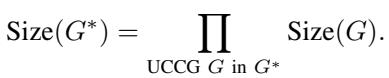
Here, \(Size(G^*)\) is the total count, and we multiply the counts of the individual components (\(G\)). The challenge, therefore, is efficiently counting the valid orientations for each UCCG.

The Clique-Picking (CP) Algorithm

This is where the 2023 “Clique-Picking” algorithm comes in. It utilizes a structure known as a Clique Tree. A chordal graph can be viewed as a tree where each node is a maximal clique (a fully connected subgraph).

The CP algorithm works recursively:

1. It picks a clique to be the root.
2. It orients edges away from this root.
3. This operation breaks the graph into smaller unconnected components.
4. It solves the problem for these smaller pieces.

While efficient compared to exponential searches, the CP algorithm has a flaw. To get the correct count, it has to iterate through every possible maximal clique acting as the root.

For a graph with \(m\) cliques, vertices \(V\), and edges \(E\), the cost of generating the sub-problems for a single root is roughly proportional to the size of the graph. Since the CP algorithm does this for every clique, the complexity hits \(\mathcal{O}(m(|V| + |E|))\).

The insight of the new paper: When you move from rooting the tree at Clique A to rooting it at Clique B, the vast majority of the graph structure does not change. The previous algorithm was blindly rebuilding the entire world for every step. The new algorithm, Super Cliques Transfer, keeps the shared structures and only updates what’s necessary.

Core Method: Super Cliques and Transfer

The authors propose a method to reduce the complexity to \(\mathcal{O}(m^2)\). This is a significant improvement, especially for dense graphs where the number of edges \(|E|\) is very large.

To understand how they achieve this, we need to define three concepts: the Clique Tree, Super Cliques, and the Transfer Operation.

1. The Rooted Clique Tree

Let’s visualize the data structure. Below, Figure 1(a) shows a graph (UCCG). Figure 1(c) shows its Clique Tree.

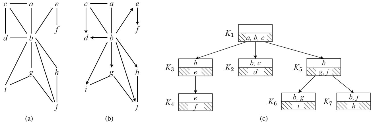
In Figure 1(c), the tree is rooted at clique \(K_1 = \{a, b, c\}\).

• \(K_1\) is the parent.
• \(K_2, K_3, K_5\) are children.
• The intersections between cliques (e.g., \(\{b, c\}\) between \(K_1\) and \(K_2\)) are called separators.
• The unique parts of a clique (e.g., \(\{d\}\) in \(K_2\) which isn’t in \(K_1\)) are called residuals.

When \(K_1\) is picked as the root, it forces orientations on the graph (Figure 1b). The undirected parts that remain (like the edge between \(g\) and \(j\)) are the sub-problems we need to solve.

2. Introducing “Super Cliques”

The authors observed that when you traverse the clique tree, certain groups of cliques behave as a single unit. They defined these units as Super Cliques.

A Super Clique is formed by a “Clique Header” and its “Clique Tails.”

• Clique Header: A clique whose separator is not a subset of its parent’s separator. It represents a structural “break” or new branch.
• Clique Tail: A descendant clique whose separator is a proper subset of the header’s separator. It essentially “follows” the header.

Why does this grouping matter? Because the residuals (the unique vertices) within a Super Clique form the specific undirected components we are trying to count.

The authors formally define a Super Residual (\(\mathrm{SR}\)) as the collection of residuals belonging to a super clique:

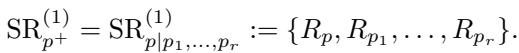
This leads to a powerful theorem. The set of Undirected Connected Components (\(\mathcal{C}_G(K_1)\)) for a rooted tree is essentially just the collection of graphs induced by these Super Residuals.

In simple terms: If you can identify the Super Cliques in the tree, you immediately identify the sub-problems you need to count. You don’t need to run a complex search algorithm on the graph vertices every time.

3. The Transfer Operation (The “Magic” Step)

Here is the core innovation. Suppose we have computed the Super Cliques for the tree rooted at \(K_1\). Now we want to know the result if we root the tree at \(K_5\).

In the standard approach, we would rebuild the tree from scratch. In this approach, we perform a Transfer.

When we move the root from parent \(K_1\) to child \(K_i\) (e.g., \(K_5\)), only the edge between them reverses direction (\(K_1 \rightarrow K_5\) becomes \(K_5 \rightarrow K_1\)).

• \(K_5\) becomes the new global root.
• \(K_1\) becomes a child of \(K_5\).
• The rest of the tree structure (siblings of \(K_5\), descendants of \(K_5\)) remains largely intact, though their status as headers or tails might shift locally.

The authors provide a lookup table (Table 1) determining exactly how the separators and residuals change during this single edge flip.

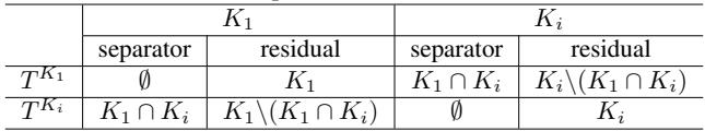
Notice how simple the update is. For most cliques, the separator and residual don’t change at all. Only the two cliques involved in the swap (\(K_1\) and \(K_i\)) see their internal sets updated.

Visualizing the Change

Let’s look at a concrete example of structure change. Figure 2 shows the transition from a tree rooted at \(K_1\) (left) to a tree rooted at \(K_5\) (right).

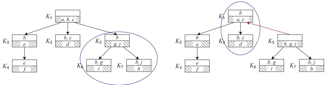
On the left (\(T^{K_1}\)):

• \(K_5\) is a child of \(K_1\).
• \(K_5\) has tails \(K_6\) and \(K_7\).
• They form a Super Clique (blue circle): \(\{K_5, K_6, K_7\}\).

On the right (\(T^{K_5}\)):

• We make \(K_5\) the root.
• The relationship with \(K_6\) and \(K_7\) breaks; \(K_6\) and \(K_7\) become their own independent Super Cliques because \(K_5\) is now the “boss” (root) and no longer acts as their header in the same way.
• However, look at \(K_1\). It is now a child of \(K_5\).
• \(K_2\) was a child of \(K_1\). It follows \(K_1\) into the new structure.
• They form a new Super Clique: \(\{K_1, K_2\}\).

The algorithm, SC-Trans, mechanizes this logic. It identifies which Super Cliques split apart and which ones merge together based on the simple subset relationships of their separators.

The updated Super Residual for the new root usually takes a form like this, merging the old root’s residual with specific tails:

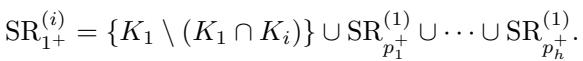
The Algorithm Workflow

The researchers implemented this logic into an iterative algorithm.

1. Initialize: Build the clique tree for the first clique \(K_1\). Find its Super Cliques.
2. Iterate: Move to an adjacent clique \(K_2\).
3. Transfer: Use the logic above to update the Super Cliques and Residuals instantly, without touching the underlying graph vertices.
4. Repeat: Traverse the whole tree until every clique has served as the root.

This workflow essentially “morphs” the tree structure step-by-step, carrying over the calculation results (\(\mathcal{C}_G\)) from neighbor to neighbor.

Experiments & Results

Does this theoretical “recycling” of structure actually save time? The authors compared their Improved Clique-Picking (ICP) algorithm against the standard Clique-Picking (CP) algorithm.

They tested on chordal graphs with varying numbers of vertices (\(V\)) and graph densities (\(r\)).

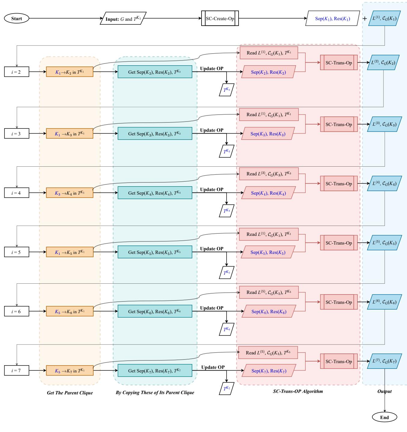
Performance on Vertex Count

In Figure 3(a) and 3(b), we see the runtime (log scale) as the number of vertices increases.

• Blue Line (ICP): The new method.
• Orange Line (CP): The standard method.

The new method is consistently faster. Note that both axes are logarithmic; a visible gap here represents a significant multiplicative speedup.

The Impact of Density

The “density” of the graph turns out to be a major factor. The table below compares the runtime difference as density (\(r\)) increases.

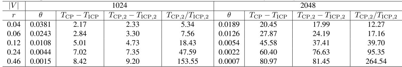
The column \(T_{CP, 2} / T_{ICP, 2}\) (the ratio of runtimes for the component-generating step) is particularly telling.

• At low density (\(r=0.04\)), the new method is ~5x faster.
• At high density (\(r=0.46\)), the new method is ~153x to 264x faster.

Why? In dense graphs, the number of cliques (\(m\)) is large, but the number of vertices (\(V\)) might be relatively small compared to the edges. The old algorithm’s complexity relied on \(|V| + |E|\), which blows up in dense graphs. The new algorithm relies on \(m^2\). By removing the dependency on vertex/edge traversal for every step, the ICP method becomes vastly superior for complex, interconnected causal structures.

Conclusion and Implications

The “Super Cliques Transfer” algorithm represents a smart evolution in graphical causal analysis. By shifting the perspective from processing raw graph vertices to manipulating high-level tree structures (Super Cliques), the authors successfully removed a major redundancy in the previous state-of-the-art approach.

Key Takeaways:

1. Don’t Recompute: In clique trees, changing the root affects the local structure significantly but leaves the global structure largely intact.
2. Super Cliques: Identifying these stable groups of cliques allows for efficient tracking of graph components.
3. Efficiency: The method reduces complexity to \(\mathcal{O}(m^2)\), making it highly scalable for dense graphs.

For students and researchers in causal inference, this work is a reminder that data structures matter. The problem of counting Markov Equivalent DAGs is mathematically heavy, but the solution came from a classic computer science principle: incremental updates are always cheaper than total re-computation. As we continue to apply causal discovery to larger, more complex datasets (like genetic networks or economic models), optimizations like this will be the engine that makes analysis feasible.