](https://deep-paper.org/en/paper/6600_copinn_cognitive_physics_-1587/images/cover.png)
Introduction
Imagine you are trying to learn a complex new subject, like calculus or a new language. If you tried to learn the most difficult concepts immediately alongside the basics, you would likely get overwhelmed and fail. Instead, humans learn best via a “curriculum”: we master the easy concepts first, building confidence and understanding, before tackling the difficult problems.
In the world of AI scientific computing, specifically Physics-Informed Neural Networks (PINNs), models often don’t have this luxury. They are typically forced to learn everything at once—simple smooth regions and complex chaotic boundaries simultaneously. This often leads to failure in critical areas.
A new research paper titled “CoPINN: Cognitive Physics-Informed Neural Networks” proposes a fascinating solution. By mimicking the human cognitive process of “easy-to-hard” learning, researchers have created a framework that drastically improves the accuracy of solving Partial Differential Equations (PDEs).
In this post, we will deconstruct how CoPINN works, why traditional methods struggle with “stubborn” data points, and how this new cognitive approach achieves state-of-the-art results.
The Problem: Unbalanced Prediction
Partial Differential Equations (PDEs) are the mathematical language of the universe. They describe heat diffusion, fluid dynamics, wave propagation, and quantum mechanics. Solving them accurately is crucial for engineering and science.
Physics-Informed Neural Networks (PINNs) have emerged as a powerful tool for this. Instead of using a mesh grid (like traditional numerical methods), PINNs use neural networks to approximate the solution, using the laws of physics (the PDE itself) as a constraint in the loss function.
The “Stubborn” Regions
However, standard PINNs have a major flaw: they treat every point in the simulation space equally.
In reality, the solution to a physics problem is rarely uniform. There are “easy” regions where the solution changes slowly and “hard” regions—often near boundaries or shock waves—where values change abruptly. When a neural network tries to minimize the average error across all points simultaneously, it tends to prioritize the easy, smooth regions because they are easier to fit. This leads to the Unbalanced Prediction Problem (UPP).
The model essentially falls into a “lazy” local minimum. It gets the general shape right but fails catastrophically at the complex boundaries.
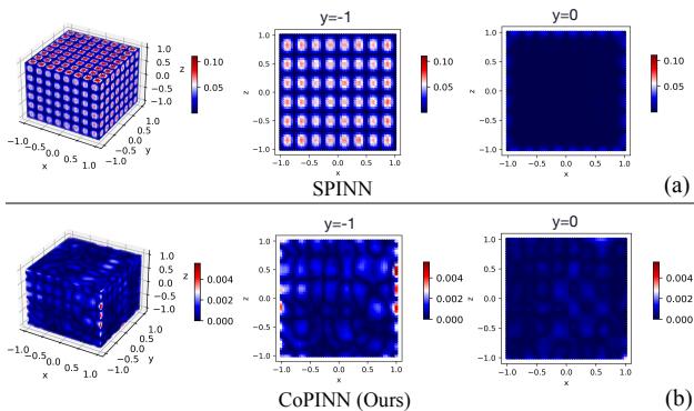
As shown in Figure 1 above, a state-of-the-art method called SPINN (Part a) exhibits massive errors (red dots) near the physical boundary (\(y = -1\)). In contrast, the proposed CoPINN (Part b) maintains consistent, low error rates across the entire domain, including the difficult boundaries.
The CoPINN Solution
To solve the UPP, the researchers introduce CoPINN. This framework integrates three key innovations:
- Separable Learning: To handle high-dimensional data efficiently.
- Difficulty Evaluation: A way for the network to self-assess which parts of the problem are “hard.”
- Cognitive Training Scheduler: A mechanism to guide the learning process from easy to hard.
Let’s look at the overall framework:
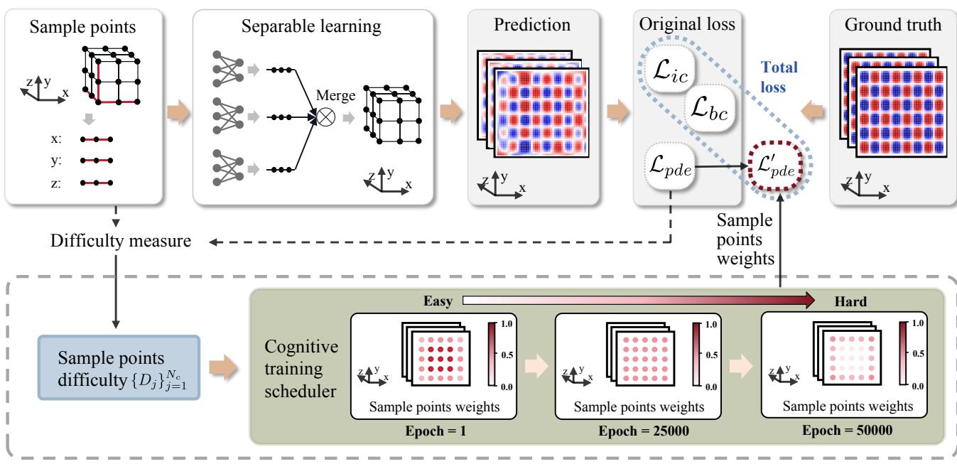
1. Separable Learning Architecture
Before tackling the “cognitive” aspect, the authors address the computational cost. Standard PINNs use a single Multi-Layer Perceptron (MLP) that takes all coordinates \((x, y, z, t)\) as input. This becomes computationally expensive as dimensions grow.
CoPINN adopts a separable architecture. Instead of one giant network, it uses independent sub-networks for each coordinate axis.
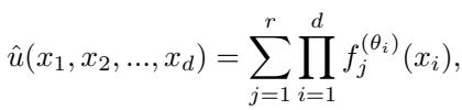
As seen in the equation above, the prediction \(\hat{u}\) is constructed by aggregating the outputs of these smaller networks via a product sum. This allows the model to process a matrix of input coordinates efficiently, significantly reducing memory usage and training time for high-dimensional PDEs.
2. Measuring Difficulty
The core of CoPINN is its ability to distinguish between “easy” and “hard” samples. But how does a neural network know what is difficult?
The researchers propose using the gradient of the PDE residuals as a proxy for difficulty.
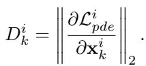
Here, \(D_k^i\) represents the difficulty of the \(k\)-th sample at epoch \(i\).
- Low Gradient: The physics loss is stable; the region is likely smooth. (Easy)
- High Gradient: The physics loss changes rapidly; this indicates a region with sharp transitions or complex boundaries. (Hard)
By calculating this dynamic difficulty score, the model can identify the “stubborn” regions that usually cause standard PINNs to fail.
3. The Cognitive Training Scheduler
This is where the “human-like” learning happens. The authors propose a scheduler inspired by Self-Paced Learning (SPL).
The goal is to optimize the loss function, which includes terms for the PDE constraints (\(\mathcal{L}_{pde}\)), Initial Conditions (\(\mathcal{L}_{ic}\)), and Boundary Conditions (\(\mathcal{L}_{bc}\)).
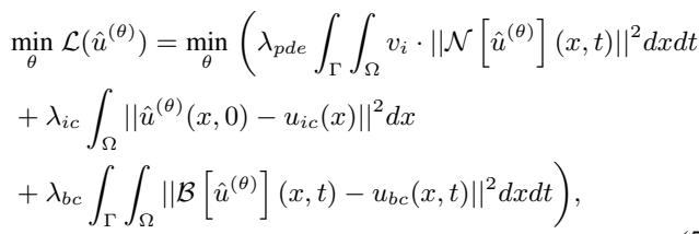
Notice the term \(v_i\) in the equation above. This is a dynamic weight assigned to each sample. The Cognitive Training Scheduler adjusts these weights over time (\(v_i\)) based on the difficulty of the sample (\(D\)).
The Curriculum Strategy
The training process is divided into stages based on epochs:
- Early Training (Warm-up): The model assigns higher weights to easy samples (\(v_e\)) and lower weights to hard samples (\(v_h\)). The network establishes a baseline understanding of the general solution structure.
- Mid Training: The weights equalize.
- Late Training: The focus shifts. The model assigns higher weights to hard samples, forcing the network to refine its predictions in the stubborn boundary regions it previously ignored.
The evolution of these weights is governed by a hyperparameter \(\beta\) and the current epoch number.
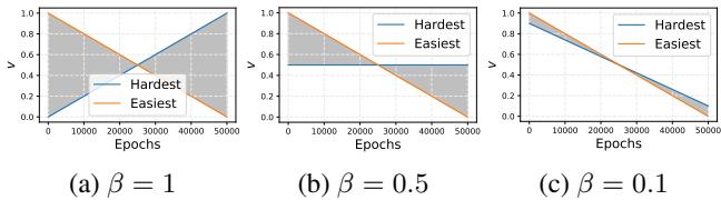
Figure 3 illustrates this shift.
- The Orange line (Easiest samples) starts with high weight (1.0) and decreases over time.
- The Blue line (Hardest samples) starts with 0 weight and increases.
- Depending on the \(\beta\) value (a hyperparameter), the crossover point changes. The authors found that a gradual shift (like in graph c) often prevents the model from forgetting what it learned earlier.
The specific formula for weighting a specific sample \(j\) at epoch \(i\) combines the global easy/hard trends with the specific difficulty of that sample:
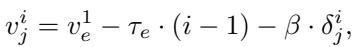
This dynamic adjustment ensures the model doesn’t get stuck in local minima caused by trying to learn complex boundaries too early.
Experiments and Results
To validate CoPINN, the researchers tested it against seven state-of-the-art baselines (including regular PINN, SPINN, and Region-Optimized PINN) on challenging physics equations:
- Helmholtz Equation
- Diffusion Equation
- Klein-Gordon Equation \(((2+1)d\) and \((3+1)d)\)
- Flow Mixing Problem
Quantitative Dominance
The results were statistically significant. Below is the table for the Helmholtz, Klein-Gordon, and Diffusion equations.
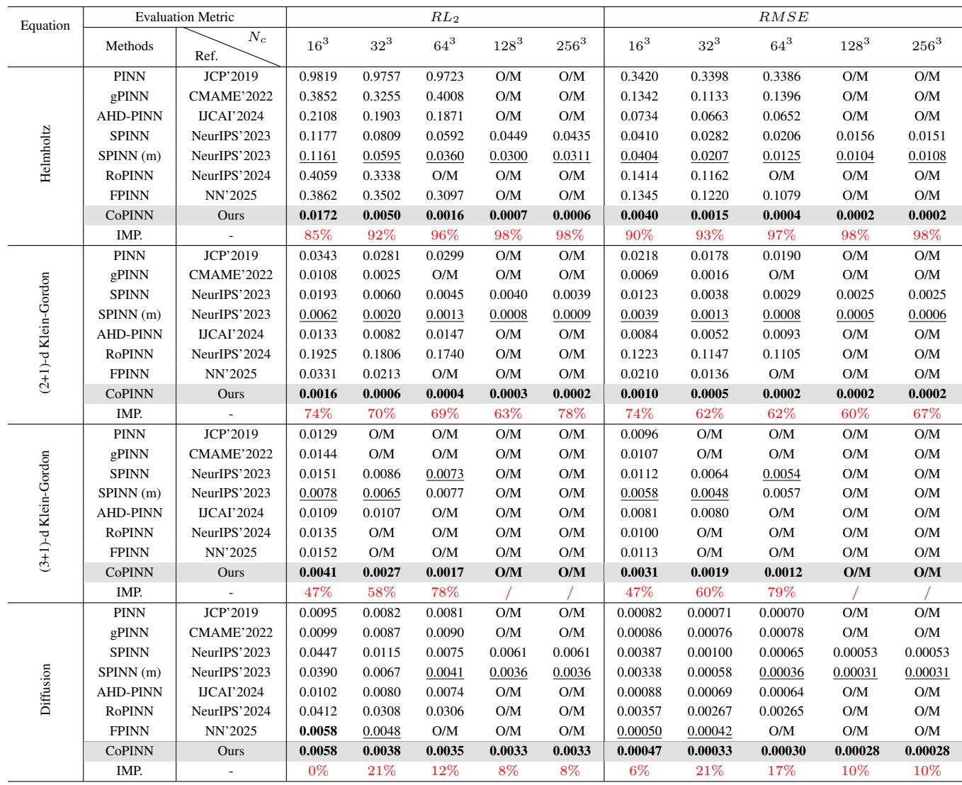
Key Takeaways from the Data:
- Helmholtz Equation: This is a particularly hard equation due to its wave-like nature. With \(256^3\) collocation points, CoPINN achieved a Relative L2 Error (\(RL_2\)) of 0.0006. The next best method (SPINN-m) scored 0.0311. That is a massive improvement in precision.
- Consistency: CoPINN achieved the best performance across almost all datasets and resolutions.
- Scalability: While many methods ran out of memory (O/M) at high resolutions (\(128^3\) and \(256^3\)), CoPINN’s separable architecture allowed it to train successfully.
Visual Analysis
Numbers are great, but visualizing the flow fields shows where the improvement happens.
Figure 4 below shows the comparison on the Helmholtz dataset. Look closely at the “Absolute Error” column.
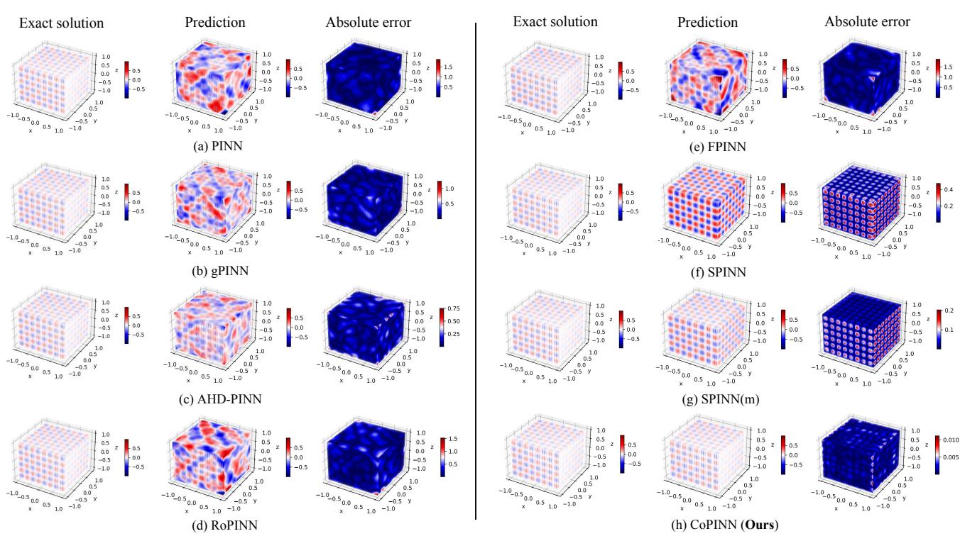
- Row (a) PINN: The error map is bright red/blue, indicating massive deviation from the exact solution.
- Row (f) SPINN: Better, but still shows significant error structures.
- Row (h) CoPINN: The error map is nearly blank (dark blue), indicating that the prediction is almost identical to the exact solution.
We see similar results for the (2+1)-d Klein-Gordon dataset:
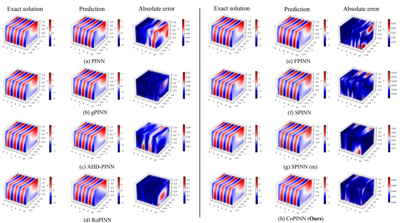
Again, CoPINN (Row h) effectively erases the error that plagues other methods (like gPINN in Row b), particularly stabilizing the learning in regions where the solution oscillates.
Convergence Stability
One might worry that changing sample weights dynamically could make training unstable. However, the error analysis shows the opposite.
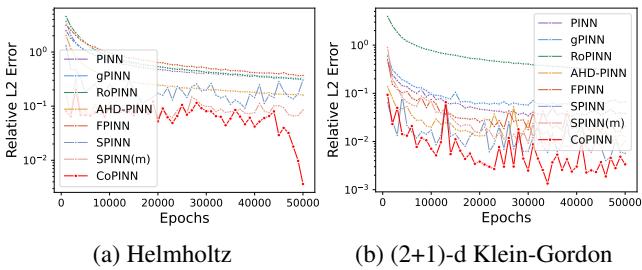
In Figure 7, the CoPINN error curve (Red) trends downward reliably. While there are small fluctuations as weights shift (which is expected in curriculum learning), the final convergence point is significantly lower than all competitors.
Conclusion
The “Unbalanced Prediction Problem” has long been a silent killer for the accuracy of Physics-Informed Neural Networks. By treating complex boundary turbulence the same as smooth internal flows, traditional models often fail where accuracy matters most.
CoPINN successfully addresses this by borrowing a page from human pedagogy: crawl before you walk, walk before you run.
By combining an efficient separable architecture with a cognitive scheduler that intelligently ramps up difficulty, CoPINN achieves:
- Higher Accuracy: Reducing errors by orders of magnitude in some cases.
- Robustness: Correctly solving stubborn boundary regions.
- Efficiency: Handling high-resolution 3D and 4D problems without running out of memory.
This research highlights that in deep learning, how a model learns is just as important as what it learns. As we apply AI to increasingly complex scientific simulations, “cognitive” strategies like self-paced learning will likely become a standard requirement for robust physics solvers.