In the world of deep learning, we often treat model parameters as a means to an end. We train them, save them, and run inference. But not all parameters are created equal. Some weights in your neural network are critical load-bearing columns; others are decorative trim that can be removed or altered without collapsing the structure.

Determining which parameters matter most is the domain of parameter sensitivity, and the “gold standard” tool for measuring this is the Fisher Information Matrix (FIM). The Fisher diagonal tells us how much the model’s output distribution would change if we perturbed a specific parameter. It is crucial for advanced techniques like Model Merging, Network Pruning, and Continual Learning.

There is just one problem: computing the Fisher is expensive. It usually requires a separate pass over the training data, calculating per-sample gradients, squaring them, and summing them up. For large language models (LLMs), this overhead can be prohibitive.

But what if you didn’t have to calculate it? What if an approximation of the Fisher was already sitting in your GPU memory, hidden in plain sight?

In the paper “Fishers for Free? Approximating the Fisher Information Matrix by Recycling the Squared Gradient Accumulator”, researchers YuXin Li, Felix Dangel, Derek Tam, and Colin Raffel propose a method called the “Squisher.” They demonstrate that the squared gradient accumulator maintained by adaptive optimizers (like Adam) can be recycled to approximate the Fisher diagonal at zero additional cost.

The Cost of Importance

To understand why the Squisher is such a useful discovery, we first need to understand the “expensive” way of doing things.

The Fisher Information Matrix (FIM)

The Fisher Information Matrix captures the curvature of the loss landscape. In simple terms, if the loss landscape is very steep around a parameter, that parameter is “important” (small changes cause large errors). If the landscape is flat, the parameter is less important.

Formally, for a neural network with parameters \(\theta\), input \(x\), and label \(y\), we look at the gradient of the log-likelihood. The standard FIM is defined as the expected covariance of the gradients:

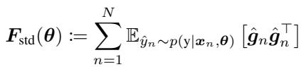
Here, \(\hat{g}_n\) represents the gradients calculated using labels sampled from the model’s own distribution.

The Empirical Fisher

In practice, sampling from the model’s distribution is tedious. Researchers often use the Empirical Fisher, which uses the ground-truth labels provided by the dataset rather than the model’s predicted distribution:

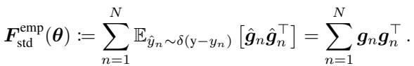
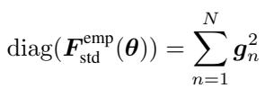
Because storing a full matrix (size \(P \times P\) where \(P\) is the number of parameters) is impossible for deep networks, we almost exclusively use the Diagonal Fisher. This simplifies the calculation to the sum of the squared gradients for each sample:

The Bottleneck

Look closely at the equation above. To compute it, you need access to the training data. You need to perform a forward and backward pass for \(N\) examples. Crucially, you need to square the gradients per sample before summing them. Most deep learning frameworks optimize for batches, averaging the gradient before you see it. Getting per-sample squared gradients usually requires inefficient loops or specialized libraries like BackPACK.

This computational friction prevents many practitioners from using powerful Fisher-based techniques.

Enter the Squisher

The authors of this paper made a keen observation: modern training doesn’t just use raw Stochastic Gradient Descent (SGD). We use adaptive optimizers like Adam, AdamW, or RMSProp.

These optimizers work by adapting the learning rate for each parameter individually. To do this, they keep track of the “second moment” of the gradients—essentially, a running average of the squared gradients.

In Adam, this accumulator, denoted as \(v^{(t)}\), is updated at every step \(t\):

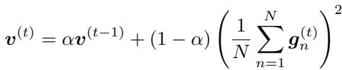
Here, \(g_n\) are the gradients in the current batch. The term in the parenthesis is the average gradient of the batch.

The Intuitive Leap

The authors asked a simple question: Is Adam’s \(v^{(t)}\) an approximation of the Fisher diagonal?

At a glance, they look similar. Both involve squaring gradients.

1. Fisher: Sum of squared gradients (\(\sum g^2\)).
2. Adam: Moving average of squared batch gradients (\(\text{Avg}(\dots (\sum g)^2 \dots)\)).

However, there is a distinct mathematical difference. The Fisher sums the squares; Adam squares the sum (of the batch). In statistics, the square of a sum is not usually the sum of squares.

To bridge this gap, the authors utilize the concept of the Joint Empirical Fisher. Instead of treating each data point as an independent random variable, if we view the entire dataset (or batch) as a joint distribution, the math shifts. The Joint Empirical Fisher is actually defined by the outer product of the aggregated gradient:

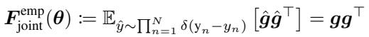
And its diagonal is simply the square of the summed gradients:

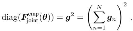
This reveals the theoretical link. The squared gradient accumulator in Adam (\(v^{(t)}\)) is essentially tracking a moving average of the Joint Empirical Fisher (scaled by the batch size).

The Squisher Recipe

The proposed method, dubbed the “Squisher” (Squared gradient accumulator as Fisher), is remarkably simple. Instead of running a complex post-training process to compute the Fisher, you simply take the optimizer state that Adam has already computed for you.

You can approximate the Fisher diagonal by recycling \(v^{(t)}\):

As shown in Figure 1, the Squisher acts as a shortcut. Instead of the computational path of “Square then Sum” (the standard Fisher), we accept the “Sum then Square” path inherent in Adam’s accumulation.

One small adjustment is required regarding scale. The standard Fisher scales with the number of datapoints \(N\). Therefore, to match the magnitude of the standard Fisher, we can scale the optimizer state:

In many applications (like ranking parameters for pruning), the absolute scale doesn’t matter, only the relative order. in those cases, you can use \(v^{(t)}\) directly.

Does it Actually Work?

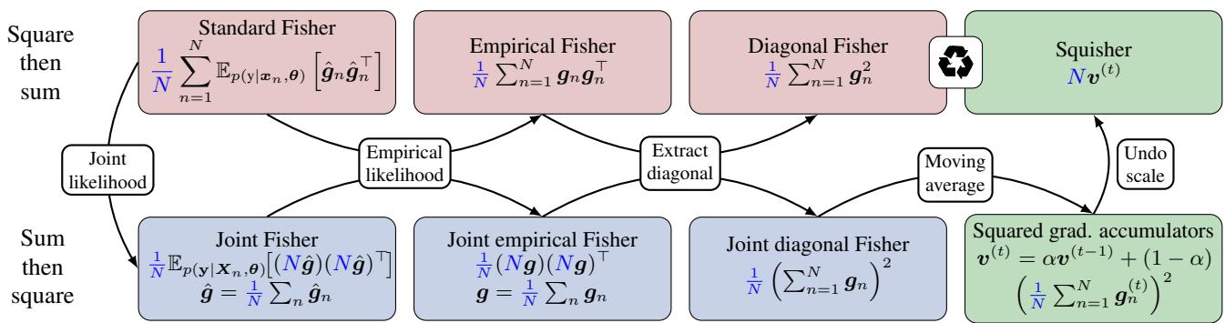
The theory is convenient, but does replacing a rigorous statistical metric (Fisher) with a “dirty” moving average (Squisher) actually work in practice? The authors tested this across five distinct applications where the Fisher diagonal is typically used.

The results were surprisingly consistent: The Squisher performs comparably to the Fisher, and both significantly outperform baselines.

Let’s look at the specific experiments.

1. Model Merging

Model merging involves combining two different fine-tuned models into one without retraining. A popular technique, Fisher Merging, takes a weighted average of the parameters. If Model A has a high Fisher value for a specific parameter (meaning it’s important), and Model B has a low value, the merged model will stay closer to Model A’s value.

The researchers tested this on T5 models fine-tuned on various text datasets.

As seen in the first panel of Figure 2, the Squisher (orange) actually performed slightly better than the standard Fisher (blue) in this setting. Both were far superior to simple averaging (Linear). Since merging relies on relative importance, the approximation holds up perfectly.

2. Uncertainty-Based Gradient Matching (UBGM)

UBGM is a more advanced merging technique that tries to align the gradient updates of multiple models. It relies heavily on the Fisher matrix to determine the direction of updates.

The update rule for UBGM is complex and relies on the inverse of the sum of Fishers:

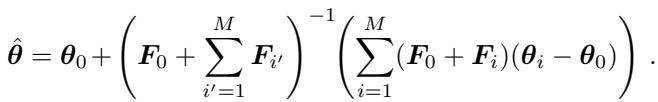
Despite this complexity, replacing the Fisher matrices \(F_i\) with the Squisher accumulators yielded nearly identical accuracy (94.00% vs 93.99%) on RoBERTa models.

3. Network Pruning

Pruning aims to remove parameters to make the network smaller and faster. The logic is simple: remove the parameters that affect the loss the least. The Fisher diagonal provides a metric for this “saliency.”

The pruning criterion using Fisher is:

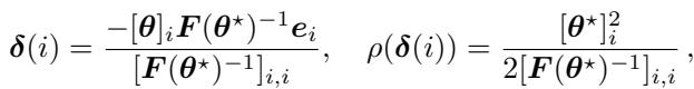
The authors pruned a VGG-13 network on CIFAR-100. Even when removing 75% of the parameters, the Squisher-based pruning remained competitive with the expensive Fisher computation, and far better than random pruning.

4. FISH Mask

Similar to pruning, “Sparse Training” involves training only a subset of parameters. The FISH Mask technique selects which parameters to train based on the Fisher diagonal.

In experiments fine-tuning BERT on GLUE benchmarks, the Squisher matched the Fisher almost exactly (within 0.1% accuracy). This confirms that the Squisher ranks parameter importance almost identically to the true Fisher.

5. Task Embeddings (Task2Vec)

We can embed an entire “task” into a vector space using the Fisher information of a model trained on that task. This helps in predicting which tasks are similar (e.g., is “Question Answering” similar to “Reading Comprehension”?).

The distance between tasks is measured using the cosine similarity of their Fisher matrices:

Using Squisher for these embeddings actually produced better results for predicting task transferability than the standard Fisher. This suggests the moving average nature of Adam might capture more robust information about the training trajectory than a static post-training calculation.

6. Continual Learning (EWC)

Finally, Elastic Weight Consolidation (EWC) prevents a model from “forgetting” old tasks when learning new ones. It does this by penalizing changes to parameters that were important for the previous task.

In this equation, \(F\) acts as the penalty weight. This is the one setting where magnitude matters. If the Squisher values are too small, the regularization is too weak; if too large, the model can’t learn the new task.

The authors found that by applying the scaling factor \(N\) (dataset size) to the Squisher, they achieved performance on par with standard EWC on Split-MNIST and CIFAR-100 benchmarks.

The “Free” Advantage

The performance results are compelling, but the real argument for the Squisher is efficiency.

Calculating the Fisher is a separate, post-training phase. It requires loading the model, loading the dataset, and performing heavy computations. The Squisher, however, is a byproduct of training. If you save your optimizer state (e.g., optimizer.state_dict() in PyTorch), you have the Squisher.

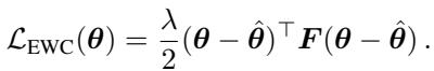
The time difference is stark:

As shown in Table 1, calculating the Fisher for Model Merging took nearly 30,000 seconds (over 8 hours). The Squisher took effectively 0 seconds. For researchers with limited compute, or for applications requiring rapid iteration, this is a game-changer.

Nuances and Limitations

Is it a perfect replacement? Not always. The authors performed ablation studies (Table 2) to understand the limits.

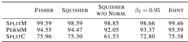
1. Scaling is Key for EWC: As noted in the “Squisher w/o Norm” column, failing to scale the accumulator by \(N\) destroys performance in Continual Learning settings where the regularization strength depends on the absolute value of the Fisher.
2. The Moving Average: The Fisher is a sum over the whole dataset. Adam is an exponential moving average (EMA). If the EMA decay rate (\(\beta_2\)) is too high or too low, the approximation might drift. However, standard Adam settings (\(\beta_2=0.999\)) work well.
3. Training Duration: For the Squisher to be accurate, the model needs to have converged sufficiently so that the running average stabilizes. In early training stages, the Squisher might be noisy.

Conclusion

The “Squisher” represents a victory for efficiency. It reminds us that the complex statistics we strive to calculate—like the Fisher Information Matrix—are often reflected in the heuristic tools we already use, like Adam.

By recognizing the mathematical link between the squared gradient accumulator and the Joint Empirical Fisher, the authors have unlocked a method to perform advanced model merging, pruning, and analysis effectively for free.

Key Takeaways for Students:

• Don’t delete your optimizer states: They contain valuable information about the geometry of the loss landscape.
• Approximations are powerful: The theoretical definition of Fisher is rigorous, but in deep learning, a “good enough” proxy like the Squisher often yields identical downstream results.
• The Fisher is versatile: From merging LLMs to preventing catastrophic forgetting, knowing which parameters matter is one of the most useful tools in the ML toolkit. Now, it’s also one of the most accessible.

So, the next time you finish training a model, don’t just save the weights. Keep the Squisher—you might get your Fishers for free.