](https://deep-paper.org/en/paper/8239_not_all_solutions_are_cre-1692/images/cover.png)
Introduction
In the quest to understand intelligence—both artificial and biological—we often rely on a fundamental assumption: if two systems perform the same task in the same way, they must be processing information similarly. If a Deep Neural Network (DNN) classifies images with the same accuracy and error patterns as a human, we are tempted to conclude that the network’s internal “neural code” aligns with the human brain.
But what if this assumption is fundamentally flawed?
A fascinating research paper titled “Not all solutions are created equal” by Braun, Grant, and Saxe challenges this foundation. The researchers dive deep into the mathematics of neural networks to prove a startling fact: Function and representation are dissociable.
You can have two networks that behave identically (same inputs, same outputs) but use completely different internal representations. Conversely, you can have networks with similar internal structures that perform different functions. This “Rashomon effect” of neural networks suggests that peering inside the “black box” is even trickier than we thought.
In this post, we will unpack this paper. We will explore the “solution manifold”—the infinite landscape of weight combinations that solve a task—and discover why some solutions are “task-specific” (reflecting the data structure) while others are “task-agnostic” (potentially hiding an invisible elephant in the weights).
The Problem of Identifiability
To understand the paper’s contribution, we first need to understand the concept of identifiability. In statistics and engineering, a system is identifiable if its internal parameters can be uniquely determined by its behavior.
Modern neural networks are heavily non-identifiable. Because they are over-parameterized (having far more neurons than strictly necessary to solve a task), there are many different combinations of weights and biases that result in the exact same input-output mapping.
This creates a massive challenge for neuroscience and AI interpretability. If we record neural activity (representations) to infer the function of a brain region, or if we analyze the hidden layers of a Transformer model to understand how it “thinks,” the non-identifiability problem suggests our findings might be arbitrary. We might be analyzing one specific version of a solution, not the solution.
The Perfect Laboratory: Deep Linear Networks
To solve this mathematically, the authors turn to Deep Linear Networks (DLNs). While modern AI uses non-linear activation functions (like ReLU or Sigmoid), DLNs use linear transformations.
\[ \hat { \mathbf { y } } _ { n } = \mathbf { W } _ { 2 } \mathbf { W } _ { 1 } \mathbf { x } _ { n } , \]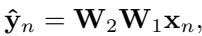
Despite their simplicity, DLNs share important properties with non-linear networks:
- They have non-convex loss landscapes (learning is complex).
- They have hidden layers that form internal representations.
- They are analytically tractable—we can solve them with exact math rather than just guessing.
The researchers analyze a two-layer linear network trained to minimize Mean Squared Error (MSE).
\[ \mathcal { L } _ { \mathrm { M S E } } = \frac { 1 } { 2 P } \sum _ { n = 1 } ^ { P } | | \hat { \mathbf { y } } _ { n } - \mathbf { y } _ { n } | | _ { 2 } ^ { 2 } \]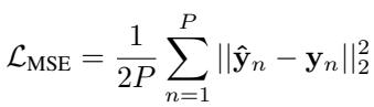
The Solution Manifold
When we train a network, we are searching for a point where the error is minimized. In over-parameterized networks, this isn’t a single point (a global minimum); it is a connected valley of optimal points called a Solution Manifold.
Imagine a flat valley floor surrounded by mountains. Every point on that floor achieves zero error (or minimum error). You can walk around this valley floor, changing your coordinates (the weights), without ever walking uphill (increasing error).
The authors demonstrate this “random walk” in Figure 1.
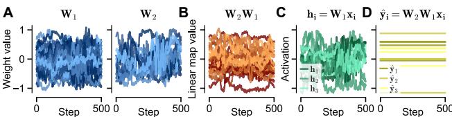
Notice panel (D) in the figure above: the network output (yellow line) never changes. However, look at (A) and (B): the weight matrices are drifting significantly. Most importantly, look at (C): the hidden-layer representations are changing.
This proves that representation drift can happen without any change in function. A neural system could effectively “rewire” itself entirely while keeping its behavior stable.
Mapping the Landscape: Four Types of Solutions
If there are infinite solutions, are they all the same? The paper categorizes the solution manifold into four distinct regions, ranging from the most flexible to the most constrained. This categorization is the theoretical heart of the paper.
The structure of the solution depends on how the network handles different subspaces of the data:
- Relevant Inputs: Information actually needed to solve the task.
- Irrelevant Inputs: Features in the input that don’t predict the output (noise or distractors).
- Null Space: Input directions that never occur in the training data.
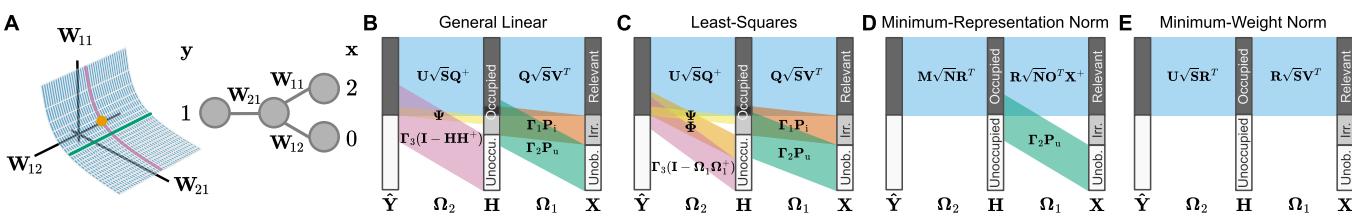
Let’s break down the four types shown in Figure 2:
1. General Linear Solution (GLS)
This is the “Wild West” of solutions. It requires only that the product of the two weight matrices (\(W_2 W_1\)) correctly maps inputs to outputs.
- Constraints: Almost none.
- Behavior: The input weights (\(W_1\)) can project irrelevant noise into the hidden layer, as long as the output weights (\(W_2\)) “cancel it out.”
- Representation: Highly arbitrary. The hidden layer can look like almost anything.
2. Least-Squares Solution (LSS)
This solution minimizes the functional norm.
- Constraints: It doesn’t react to “ghost” inputs (inputs that never exist).
- Behavior: It still processes irrelevant features present in the training data.
- Representation: Still highly flexible and Task-Agnostic.
3. Minimum Representation-Norm Solution (MRNS)
This solution minimizes the energy (norm) of the hidden layer activity.
- Constraints: Strict. It filters out all irrelevant information immediately at the first layer.
- Behavior: The hidden layer contains only the information strictly necessary to solve the task.
- Representation: Unique (up to rotation) and Task-Specific.
4. Minimum Weight-Norm Solution (MWNS)
This minimizes the size of the weights themselves (often achieved by weight decay regularization).
- Constraints: Balanced. It distributes the “work” equally between the input and output layers.
- Representation: Unique and Task-Specific.
The Elephant in the Room: Hidden Representations
Here is where the math translates into a striking conceptual finding. Because GLS and LSS (the flexible solutions) are Task-Agnostic, their internal representations don’t have to look like the task. In fact, they can look like anything you want.
To prove this, the authors designed a “semantic hierarchy” task (classifying items like plants, animals, objects). They then mathematically forced a GLS network to solve the task perfectly, but with a specific constraint: make the hidden layer activity look like an elephant.
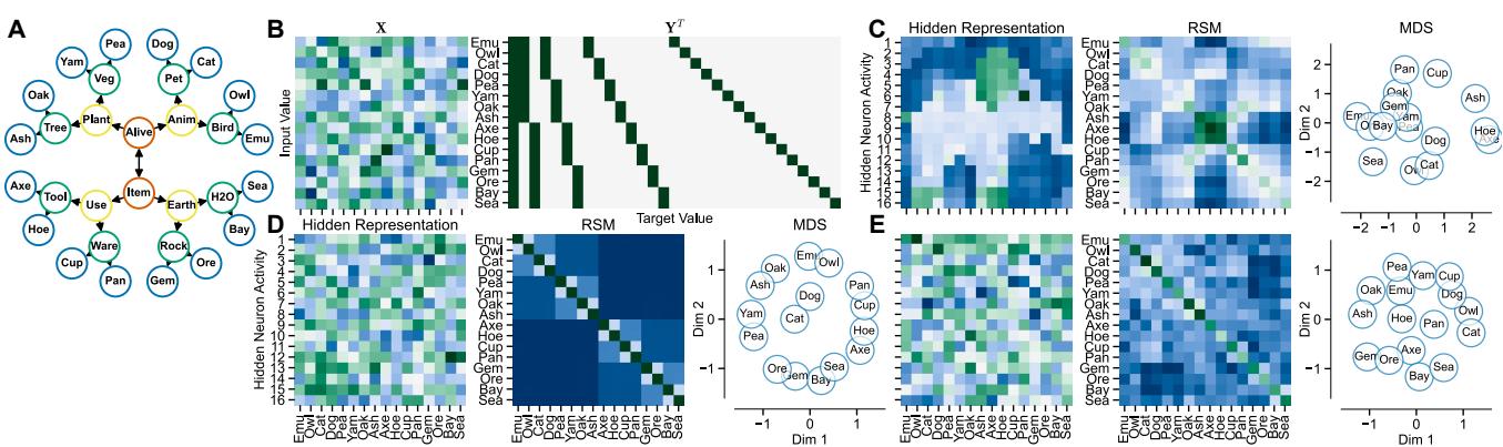
Look at Figure 3:
- Row C (GLS): The hidden representation (left plot) literally forms the shape of an elephant. The Representational Similarity Matrix (RSM) in the middle looks like a grid—it has no structure related to the task. Yet, this network solves the task perfectly.
- Row D (MRNS): The hidden representation appears random to the eye, but the RSM reveals a blocky, hierarchical structure. The network effectively “grouped” similar concepts (animals with animals, plants with plants) in its brain.
- Row E (MWNS): Similar to MRNS, it shows strong task-related structure.
The Takeaway: If you analyze a network (or a brain) and find a messy or weird representation, it doesn’t mean the system isn’t working. Conversely, you can have two systems solving the same problem where one organizes data hierarchically (Task-Specific) and the other organizes data in the shape of an elephant (Task-Agnostic).
Implications for Neuroscience and AI Evaluation
This dissociation has massive implications for how we compare artificial networks to biological brains. Two common techniques are Linear Predictivity (can I predict one network’s activity from another?) and Representational Similarity Analysis (RSA) (do both networks think “dog” and “cat” are similar?).
The authors ran simulations to see how these metrics hold up across different solution types.
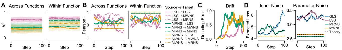
Linear Predictivity (Figure 4A)
- Result: You can easily predict a Task-Specific representation from a Task-Agnostic one (because the agnostic one has extra degrees of freedom).
- Problem: You generally cannot predict a Task-Agnostic representation from a Task-Specific one.
- Conclusion: Low predictivity might not mean functional difference; it might just mean one network is “lazier” (GLS) and carrying more useless information than the other.
RSA Correlation (Figure 4B)
- Result: When comparing Task-Agnostic solutions (GLS/LSS), the RSA correlation fluctuates wildly (the squiggly lines).
- Conclusion: If you use RSA to compare two networks that haven’t been constrained to be efficient (Task-Specific), your results are essentially random. You are measuring the “elephant,” not the function.
Drifting Representations (Figure 4C)
- Result: If a system drifts along the solution manifold (random walk), a decoder trained at Time 0 will fail at Time 100, even though the network’s behavior hasn’t changed.
- Conclusion: “Representational Drift” in the brain might not be learning or forgetting; it might just be a random walk on the manifold of equivalent solutions.
What Drives the System? The Role of Noise
If infinite solutions exist, why do biological brains (and many artificial networks) seem to converge on structured, task-specific representations? Why don’t we see “elephant-shaped” representations in the visual cortex?
The authors test three hypotheses:
- Generalization: Maybe task-specific representations are better at generalizing to new data?
- Finding: No. The paper proves analytically that generalization error does not constrain the representation to be task-specific.
- Input Noise: Maybe the system needs to be robust to noisy sensory data?
- Finding: No. Robustness to input noise leads to the LSS (Least-Squares Solution). As we saw, LSS is task-agnostic. It cleans up the output but allows messy internal representations.
- Parameter Noise: Maybe the system needs to be robust to synaptic jitter (noisy weights)?
- Finding: Yes.
The authors derive the expected loss under parameter noise:
\[ \begin{array} { r l r } { { \frac { 1 } { 2 P } \sum _ { n = 1 } ^ { P } | | ( \Omega _ { 2 } + \Xi _ { 2 } ) ( \Omega _ { 1 } + \Xi _ { 1 } ) ( \mathbf { x } _ { n } + \pmb { \xi } _ { \mathbf { x } _ { n } } ) - \mathbf { y } _ { n } | | _ { 2 } ^ { 2 } } } \\ & { } & \\ & { } & { = \frac { \sigma _ { \mathbf { x } } ^ { 2 } } { 2 } \big ( | | \Omega _ { 2 } \Omega _ { 1 } | | _ { F } ^ { 2 } + | | \Omega _ { 2 } | | _ { F } ^ { 2 } + | | \Omega _ { 1 } | | _ { F } ^ { 2 } \big ) \qquad ( 2 9 . } \\ & { } & \\ & { } & { \qquad + \frac { 1 } { 2 P } \big ( | | \Omega _ { 2 } | | _ { F } ^ { 2 } + | | \Omega _ { 1 } \mathbf { X } | | _ { F } ^ { 2 } \big ) + c , } \end{array} \]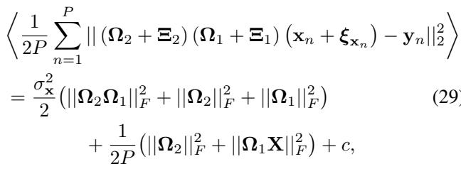
This equation shows that to minimize error under parameter noise, the network must minimize the norms of the weights (\(\|\Omega\|_F^2\)) and the hidden activity (\(\|\Omega_1 X\|_F^2\)).
Conclusion: Systems that are robust to synaptic noise (or heavily regularized artificial nets) are forced into the MRNS/MWNS regime. They must discard irrelevant info. This pressure aligns the representation with the task.
Beyond Linear: Non-Linear Networks
Finally, one might ask: “Does this apply to modern deep learning with ReLUs and Convolutions?”
The authors show that while non-linear networks are harder to solve analytically, the logic holds. They trained a standard ReLU network on MNIST (digit recognition) and then used “function-preserving transformations” to distort the hidden layer without changing the predictions.
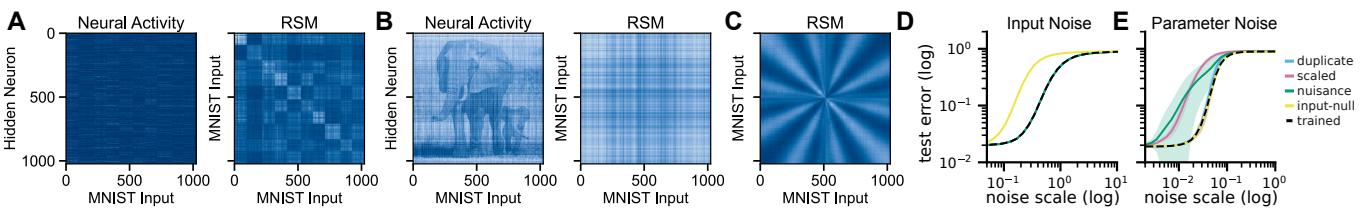
As shown in Figure 5, they could take a standard MNIST network (Panel A) and effectively “inject” an elephant into its hidden representations (Panel B) without changing a single classification.
However, just like in the linear case, the “expanded” (messy) networks were highly sensitive to parameter noise (Panel E, blue/pink lines), while the minimal, task-trained network (black line) was robust.
Summary and Final Thoughts
This paper provides a rigorous mathematical warning against conflating what a network does with how a network thinks.
- The Dissociation: A network’s function does not dictate its internal representation. Infinite variations exist.
- The Trap: Task-agnostic solutions (GLS) can hide arbitrary information (like elephants) in their weights, rendering standard comparison tools (RSA) unreliable.
- The Constraint: Robustness to parameter noise (synaptic stability) is the key constraint that forces representations to align with the task structure.
For students of machine learning and neuroscience, this suggests that “representation learning” is not just about solving the task. It’s about solving the task efficiently in the face of internal noise. Without that constraint, the ghost in the machine could look like anything at all.