Introduction

Imagine trying to predict the motion of a complex system, like a set of pendulums connected by springs, or charged particles bouncing around in a box. In physics and engineering, these are known as Coupled Dynamical Systems. To model them, we don’t just look at one object in isolation; we have to account for how every component interacts with every other component over time.

For years, scientists used handcrafted differential equations to solve these problems. But recently, Deep Learning has entered the chat. Specifically, a framework called Graph Ordinary Differential Equations (GraphODE) has shown immense promise. By combining Graph Neural Networks (GNNs) to model interactions and ODE solvers to model time, these networks can theoretically learn the “laws of physics” directly from data.

But there is a catch.

Most existing GraphODE models cheat. Instead of learning universal physical laws (like Newton’s laws or Coulomb’s law), they tend to memorize the specific context of their training data. If you train them on a system with specific material properties or interaction strengths, they fail spectacularly when you test them on a system with slightly different conditions.

In this post, we are diving deep into a paper titled “Rethink GraphODE Generalization within Coupled Dynamical System”. The researchers propose a new framework called GREAT (Generalizable GraphODE with disentanglement and regularization). They apply a causal lens to the problem, identifying exactly why current models fail to generalize and offering a sophisticated mathematical solution to fix it.

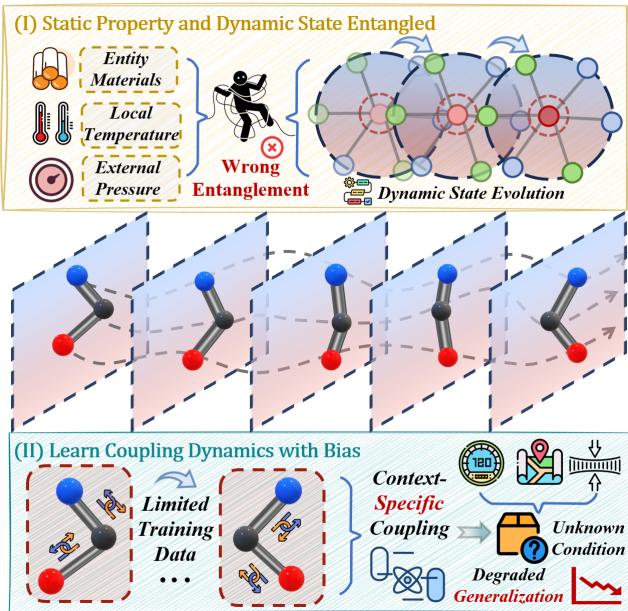
As illustrated in Figure 1 above, the core problem is twofold:

1. Entanglement: The model confuses static properties (like mass or material) with dynamic states (like velocity).
2. Spurious Coupling: The model overfits to the specific interaction patterns in the training set, rather than learning the underlying rule of interaction.

Let’s explore how GREAT solves this.

Background: The graphODE Framework

To understand the solution, we first need to understand the baseline. A coupled dynamical system is essentially a graph that changes over time. Nodes represent entities (like particles), and edges represent interactions (like forces).

In a standard Neural ODE, the evolution of a node’s state \(h_i(t)\) is governed by a function \(g_\theta\) (a neural network). This network looks at the node’s current state and the states of its neighbors:

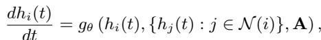
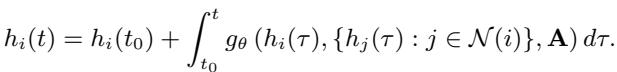
Here, \(\mathcal{N}(i)\) represents the neighbors of node \(i\), and \(\mathbf{A}\) is the adjacency matrix defining the graph structure. To find the state of the system at any future time \(t\), we start from an initial state \(h_i(t_0)\) and integrate this differential equation:

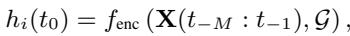
The initial state itself is usually learned by an encoder network that looks at a short history of observations:

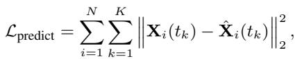
Finally, the model is trained by minimizing the difference between the predicted trajectory and the actual ground truth trajectory:

While this setup works beautifully for “in-distribution” data (data that looks exactly like the training set), it breaks down when the physical parameters change. The researchers argue that this breakage happens because the model lacks a causal understanding of the system.

A Causal Perspective

The authors introduce a Structural Causal Model (SCM) to analyze the system. An SCM allows us to draw a diagram of how variables influence each other and identify “backdoor paths”—spurious correlations that mislead the model.

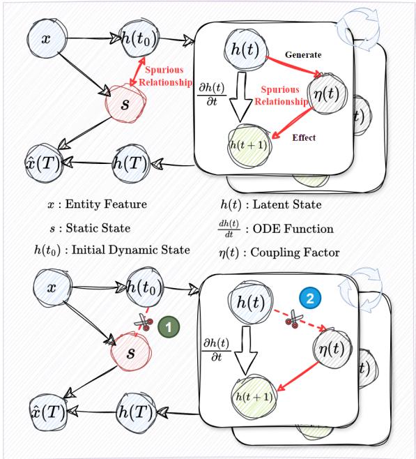
Figure 2 highlights the two critical flaws in standard GraphODEs:

1. The Static Confounder (\(x \to s \to h(t)\)): The input features \(x\) contain both static info (e.g., mass) and dynamic info (e.g., velocity). The static info \(s\) should only influence the initial setup. However, standard encoders mix \(s\) into the dynamic state evolution \(h(t) \to h(t+1)\). If the model relies on static “shortcuts” to predict movement, it fails when those static properties change.
2. The Coupling Confounder (\(h(t) \to \eta(t) \to h(t+1)\)): The coupling factor \(\eta(t)\) represents the strength of interaction. In training, specific states might correlate with specific coupling strengths purely by chance or context. The model learns this bias instead of the universal interaction law.

To build a Generalizable GraphODE, the authors propose a new governing equation that explicitly includes a coupling factor \(\eta_{i,j}(t)\):

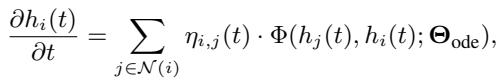
Here, the goal is to learn \(\Theta_{ode}\) (the physical law) such that it holds true regardless of the specific context.

The GREAT Method

The GREAT framework (Generalizable GraphODE with disentanglement and regularization) addresses the two causal flaws using two distinct modules.

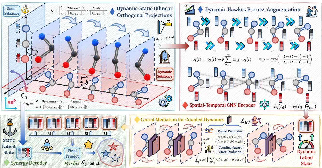
As shown in the architecture diagram (Figure 3), the workflow is split into:

1. DyStaED (Top Left): Decoupling static and dynamic states.
2. CMCD (Bottom Right): Causal mediation to fix coupling biases.

Let’s break these down.

1. Dynamic-Static Equilibrium Decoupler (DyStaED)

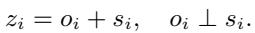
The first step is ensuring that “what an object is” doesn’t get confused with “what an object is doing.” The encoder produces a latent state \(z_i\). The authors aim to decompose this into two orthogonal components: a dynamic part \(o_i\) and a static part \(s_i\).

Orthogonal Subspace Projection

To achieve this separation mathematically, the model learns two specific subspaces (coordinate systems): one for static features and one for dynamic features.

The model projects the latent state \(z_i\) onto these subspaces. Think of this like taking a vector in 3D space and separating it into its X-axis component and its Y-axis component.

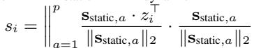
The static component \(s_i\) is calculated by projecting \(z_i\) onto the static basis vectors:

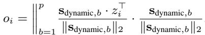
Similarly, the dynamic component \(o_i\) is found using the dynamic basis vectors:

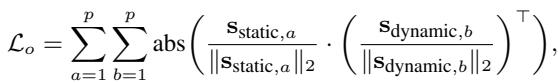
To ensure these two components are truly distinct and don’t share information, the authors impose an Orthogonality Loss. This forces the static and dynamic subspaces to be perpendicular (cosine similarity of 0).

Dynamic Hawkes Process Augmentation

Separating the states isn’t quite enough. Physical systems have “inertia” or history—past states influence the present. To capture this self-exciting nature, the authors augment the dynamic state using a Hawkes Process. This mechanism allows the current dynamic state to be influenced by a weighted sum of its history.

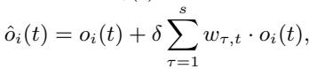
The weights decay over time, meaning recent history matters more than distant history:

This results in a robust initial state \(h_i(t_0)\) that contains rich dynamic information but is clean of static attributes.

2. Causal Mediation for Coupled Dynamics (CMCD)

Now that we have a clean dynamic state, we need to solve the second problem: biased coupling. We want the model to learn how objects interact based on universal rules, not based on the specific context of the training data.

In causal terms, we want to perform an intervention. We want to ask: “What happens to the system if we set the initial state, removing the influence of spurious coupling correlations?”

Mathematically, the researchers want to estimate the probability of the trajectory given an intervention on the initial state, denoted as \(do(h_i(t_0))\). This is difficult because the “true” coupling factor \(\eta\) is unobserved (latent).

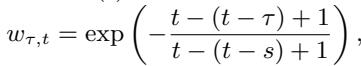
Variational Inference

The authors tackle this using variational inference. They treat the coupling factor \(\eta_i(t)\) as a latent variable. They derive a training objective (Evidence Lower Bound or ELBO) that tries to reconstruct the trajectory while regularizing the coupling factor.

The core idea is to approximate the true coupling distribution using a simpler distribution \(q\). The derivation leads to a loss function that includes a KL Divergence term:

This KL term forces the learned coupling distribution \(q(\eta_i(t) | h_i(t))\) to be close to a “context-agnostic” prior \(p(\eta_i(t))\). Essentially, it prevents the model from overfitting the coupling logic to the specific training scenario.

Factor Estimator and Evolution

But how do we actually get the value of the coupling factor \(\eta\)? The model estimates it from the dynamic state using a Gumbel-Softmax approach. This allows the model to sample discrete coupling “modes” while remaining differentiable (so we can train it with backpropagation).

Finally, to allow for complex, periodic behaviors (like springs oscillating), the dynamic state is decomposed into trigonometric sub-states (sine and cosine components).

The final differential equation that the solver integrates looks like this:

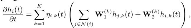
Here, the state evolution is a weighted sum of interactions, modulated by the learned, causal coupling factor \(\eta_{i,k}(t)\).

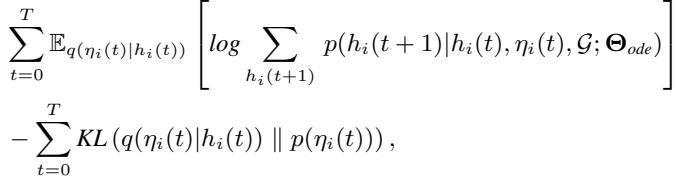
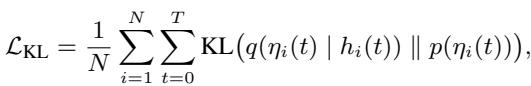
The Total Loss Function

The model is trained end-to-end using a combined loss function:

This combines:

1. Prediction Accuracy (\(\mathcal{L}_{predict}\)): Does the trajectory match reality?
2. Causal Regularization (\(\mathcal{L}_{KL}\)): Is the coupling logic unbiased?
3. Disentanglement (\(\mathcal{L}_{o}\)): Are static and dynamic states separated?

Experiments and Results

The authors tested GREAT on three physics-based datasets:

1. SPRING: Masses connected by springs (Hooke’s law).
2. CHARGED: Charged particles interacting via Coulomb forces.
3. PENDULUM: A chain of connected pendulums.

They evaluated two settings:

• In-Distribution (ID): Test data has the same parameter ranges as training data.
• Out-of-Distribution (OOD): Test data has different parameters (e.g., heavier masses, stronger charges, different initial velocities) to test generalization.

Performance Comparison

Table 1 below shows the results (RMSE is Root Mean Square Error, lower is better).

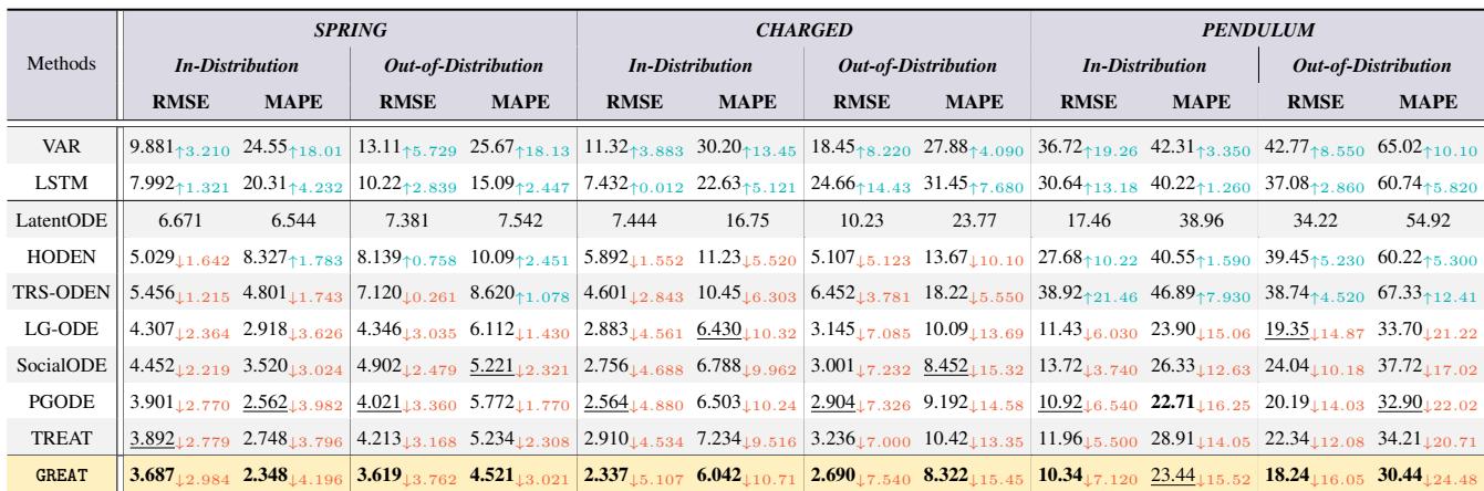
Key Takeaways:

• Dominance: GREAT achieves the best performance (bold) in almost every category.
• OOD Generalization: The gap between GREAT and other models (like LG-ODE or TREAT) is massive in the Out-of-Distribution columns. This proves that the causal disentanglement allows the model to adapt to new physical environments much better than standard approaches.

Visualizing Trajectories

Numbers are good, but seeing is believing. Figure 4 visualizes the predicted paths of particles in the SPRING dataset (OOD setting).

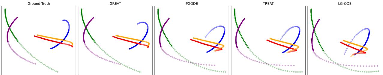
• Ground Truth (Left): The actual path.
• GREAT (2nd from Left): Almost perfectly overlaps the ground truth.
• Competitors (Right): Notice how TREAT and LG-ODE diverge significantly from the true path. They “learned” the wrong physics during training and couldn’t adapt to the OOD parameters.

Do the Components Matter? (Ablation Study)

The authors also checked if both the Decoupler (DyStaED) and the Causal Mediation (CMCD) were necessary.

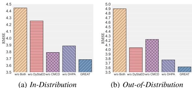
Figure 5 shows that removing either component increases the error (RMSE).

• w/o DyStaED: Removing the static/dynamic split hurts performance.
• w/o CMCD: Removing the causal coupling regularization hurts even more, especially in OOD settings.
• w/o Both: The error skyrockets.

Long-Term Prediction

Finally, they tested how well the model predicts far into the future.

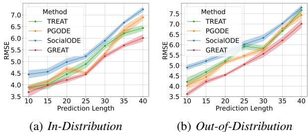
Figure 6 shows that as the prediction horizon increases (X-axis), the error for all models goes up (which is expected in chaos theory). However, GREAT (red line) maintains a much lower error rate compared to others, exhibiting superior stability.

Conclusion

The GREAT paper presents a significant step forward in combining Deep Learning with scientific modeling. By treating the learning process as a causal inference problem rather than just curve fitting, the authors managed to build a model that doesn’t just memorize data—it begins to understand the underlying mechanics.

The two key innovations—DyStaED for separating “what things are” from “how things move,” and CMCD for learning unbiased interaction rules—allow the model to generalize to new environments in ways that traditional GraphODEs cannot.

For students and researchers in AI for Science, this highlights a crucial lesson: When modeling the physical world, architecture alone isn’t enough. We must carefully consider the causal structure of our variables to ensure our models learn the laws of nature, not just the biases of our datasets.