Introduction: The Problem with Randomness

Imagine trying to learn a new language. You wouldn’t start by trying to write a complex dissertation on philosophy. You would start with the alphabet, then simple words, then sentences, and finally, complex paragraphs. This progression—from easy to hard—is fundamental to human learning. It builds confidence and ensures that foundational concepts are mastered before tackling difficult ones.

In the world of Machine Learning, specifically Graph Neural Networks (GNNs), this concept is often ignored.

Graph-structured data is everywhere—social networks, chemical molecules, and citation maps. To analyze this data without expensive human labeling, researchers use Self-Supervised Learning (SSL). A popular approach within SSL is the Masked Graph Autoencoder. The idea is simple: hide (mask) parts of the graph, and ask the AI to guess what’s missing. If it can reconstruct the missing pieces, it “understands” the graph.

However, most existing methods mask the graph randomly. They treat every edge and node as equally difficult to reconstruct. This is like handing a calculus exam to a kindergarten student one day and an alphabet worksheet to a university student the next.

This blog post explores a fascinating research paper, “Self-supervised Masked Graph Autoencoder via Structure-aware Curriculum,” which introduces Cur-MGAE. This new framework teaches GNNs using a curriculum—starting with easy patterns and gradually introducing complex structural dependencies.

Background: Graphs, Masking, and Self-Supervision

Before diving into the new method, let’s establish the context.

The Challenge of Labels

Deep learning models are data-hungry. In supervised learning, every piece of data needs a label (e.g., “this node is a bot,” “this node is a human”). Getting these labels is expensive and time-consuming. Self-supervised learning (SSL) solves this by creating “pretext tasks”—training the model on the data itself without external labels.

Generative vs. Contrastive

There are two main flavors of Graph SSL:

1. Contrastive: The model learns to distinguish between a graph and a corrupted version of itself. While powerful, it relies heavily on “augmentations” (ways to tweak the graph) that can be tricky to design.
2. Generative: The model acts like a detective. We remove parts of the graph (edges or node features), and the model tries to regenerate them. This is where our focus lies today.

The Curriculum Gap

Existing generative models, like GraphMAE, have shown great success. However, they lack nuance. In a real graph, some edges are obvious (e.g., a connection between two very similar papers), while others are surprising or complex. By treating all edges as equal, standard models suffer from suboptimal learning. They might get overwhelmed by hard samples early in training or bored by easy samples later on.

The Core Method: Cur-MGAE

The researchers propose Cur-MGAE (Curriculum Masked Graph Autoencoder). The goal is to capture the underlying difficulty of edges and design a reconstruction task that scales with the model’s capability.

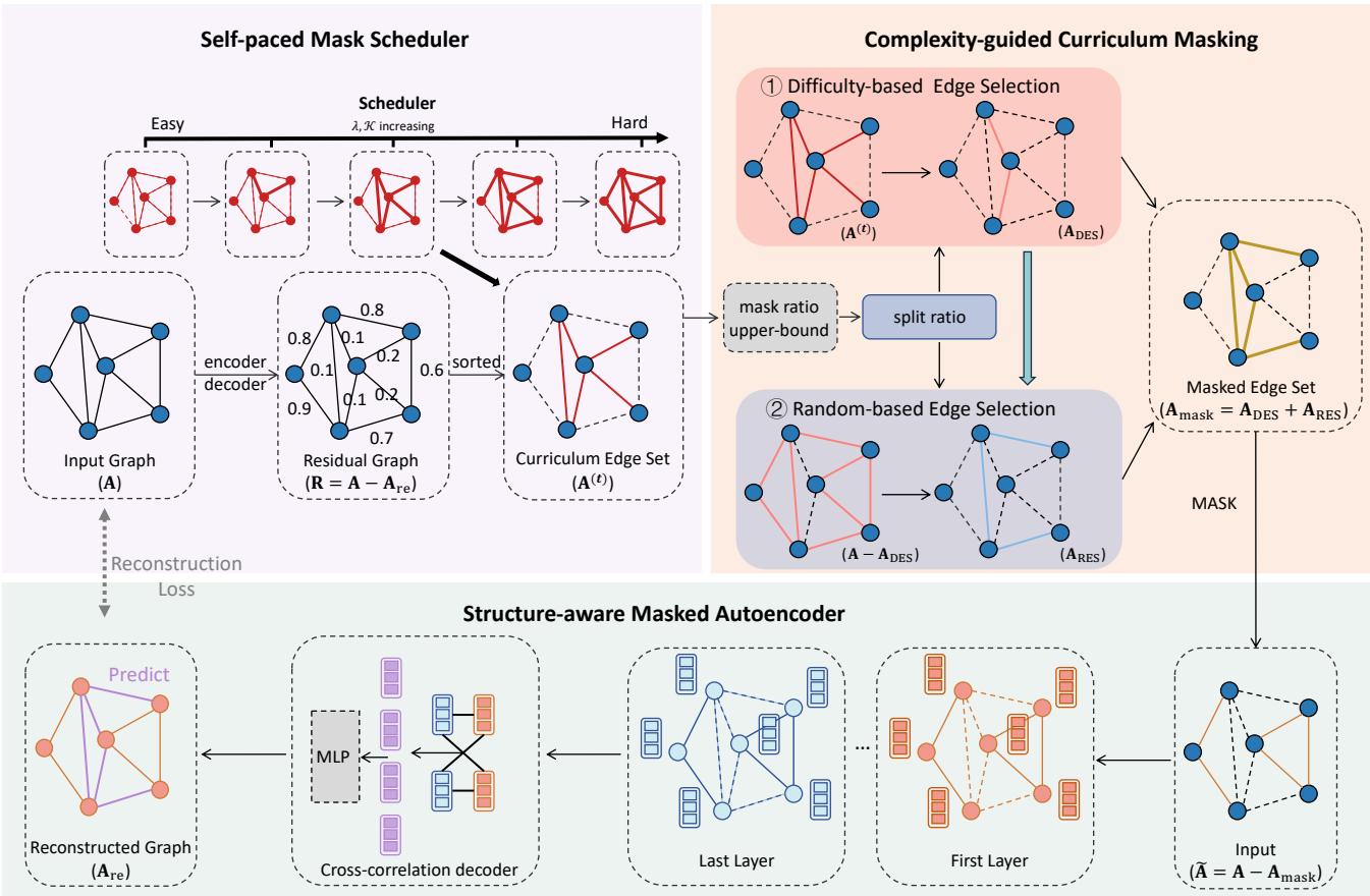
As shown in Figure 1 above, the framework consists of three integrated components:

1. Structure-aware Masked Autoencoder: The engine that learns representations.
2. Complexity-guided Curriculum Masking: The “teacher” that decides which edges are easy or hard.
3. Self-paced Mask Scheduler: The “scheduler” that decides when to introduce harder tasks.

Let’s break these down step-by-step.

1. Structure-aware Masked Autoencoder

The heart of the system is the autoencoder. It takes a graph with some edges removed (masked) and tries to predict where those edges should be.

The Encoder The encoder is a standard Graph Neural Network (like a GCN or GraphSAGE). It aggregates information from a node’s neighbors to create a “node embedding”—a numerical vector representing that node.

Here, \(h_v^{(k)}\) is the embedding of node \(v\) at layer \(k\). The function aggregates messages from neighbors (\(N_v\)) and combines them with the node’s previous state.

The Cross-Correlation Decoder Most previous models simply take the dot product of two node embeddings to see if they should be connected. The authors of Cur-MGAE argue this is too simple. Instead, they propose a Cross-correlation Decoder.

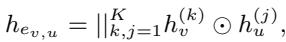
This formula looks complex, but the intuition is straightforward: instead of just checking if two nodes are similar, the decoder looks at the element-wise interaction (\(\odot\)) between nodes across different layers of the network. This captures shared features more effectively, filtering out noise and focusing on the strong signals that indicate a connection.

The Reconstruction Loss The model learns by minimizing the difference between its predictions and the actual graph structure.

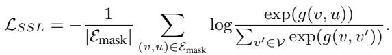
This loss function (\(L_{SSL}\)) forces the model to assign a high probability to the edges that were masked (\(E_{mask}\)), ensuring the learned representations capture the graph’s true structure.

2. Complexity-guided Curriculum Masking

This is where the “Curriculum” begins. How do we determine if an edge is “easy” or “hard” to reconstruct?

The authors use a clever, dynamic metric: Reconstruction Residual.

1. The model tries to reconstruct the entire graph using its current knowledge.
2. We calculate the error (residual) for every edge.

• Low Residual: The model predicted this edge easily. It is an “easy” edge.
• High Residual: The model struggled to predict this. It is a “hard” edge.

The strategy is counter-intuitive but brilliant: Mask the easy edges first.

Why? Because if you mask a “hard” edge (one the model creates high error on even when it is present), the model has no context to guess it. By masking the “easy” edges (those the model is confident about), you allow the model to practice on tasks it can actually solve, solidifying its basic understanding before moving on.

3. Self-paced Mask Scheduler

We cannot stick to easy edges forever. To learn robustly, the model must eventually tackle the difficult ones. The Self-paced Mask Scheduler manages this transition.

The researchers treat edge selection as an optimization problem. They want to select a set of edges to mask (represented by matrix \(\mathbf{S}\)) that balances the current difficulty with a regularization term.

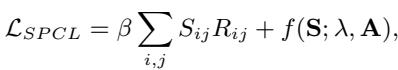
• \(R_{ij}\) is the residual (difficulty).
• \(S_{ij}\) is the selection (1 if we mask it, 0 if we don’t).
• \(f(\mathbf{S}; \lambda, \mathbf{A})\) is a regularizer controlled by \(\lambda\).

The Role of Lambda (\(\lambda\)) The parameter \(\lambda\) is the throttle. As training progresses, \(\lambda\) is increased. A higher \(\lambda\) encourages the model to select more edges, and importantly, edges with higher difficulty scores.

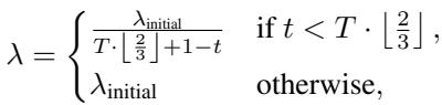
This equation ensures a smooth ramp-up. Early in training (\(t\) is small), \(\lambda\) is small, so we only pick the easiest edges. As \(t\) approaches the total epochs \(T\), \(\lambda\) grows, forcing the model to mask and reconstruct increasingly complex parts of the graph.

Balancing Exploration and Exploitation

If we only picked edges based on difficulty, the model might overfit to specific patterns. To prevent this, the authors introduce a Split Ratio.

• Difficulty-based Selection (\(A_{DES}\)): A portion of edges are selected because they fit the current curriculum difficulty.
• Random Selection (\(A_{RES}\)): The remaining edges are selected randomly.

This mix ensures the model follows a curriculum while maintaining enough randomness to explore the whole graph structure effectively.

The Unified Objective

Finally, the model optimizes both the self-supervised reconstruction and the curriculum schedule simultaneously.

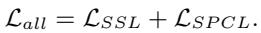
This leads to a bi-level optimization problem, where the model parameters and the masking strategy evolve together in harmony.

Experiments and Results

Does teaching an AI “easy-to-hard” actually work? The authors tested Cur-MGAE on several benchmark datasets (Cora, Citeseer, PubMed, OGB) against strong baselines like GraphMAE, MaskGAE, and contrastive methods like DGI.

1. Node Classification

In this task, the model learns representations without labels, and a simple classifier is then trained on top to predict node categories.

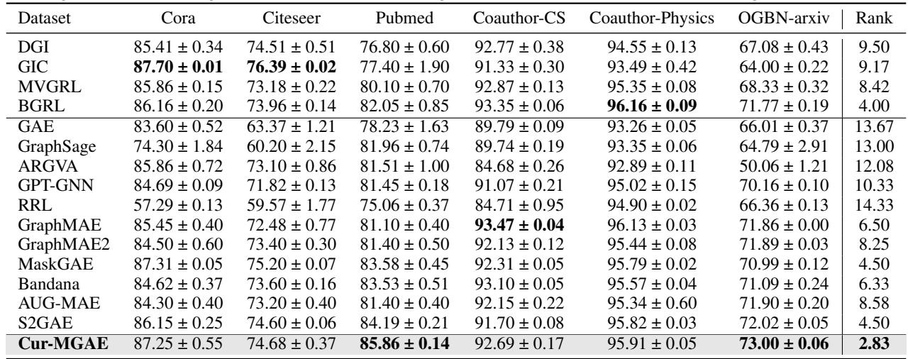
The Verdict: Cur-MGAE achieves the best average rank across all datasets. On the PubMed dataset, it improved accuracy by 1.67% over the strongest baseline. This confirms that the curriculum helps the encoder learn more discriminative features that are useful for classification.

2. Link Prediction

Here, the model must predict missing connections in a graph—a task directly aligned with the pre-training objective.

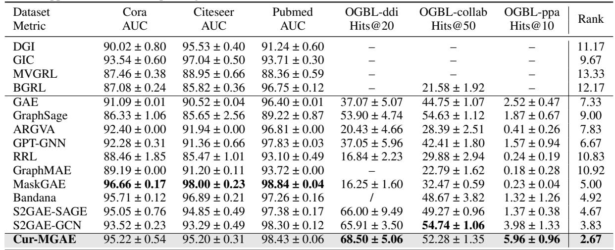
The Verdict: Again, Cur-MGAE shows consistent superiority, particularly on large-scale datasets like OGBL-ppa. Generative models generally beat contrastive ones here, but Cur-MGAE’s ability to adaptively select training samples gives it the edge over other generative models like MaskGAE.

3. Visualizing the Curriculum

To prove the model is actually learning “Easy-to-Hard,” the researchers created a synthetic dataset where they knew the ground-truth difficulty of every edge.

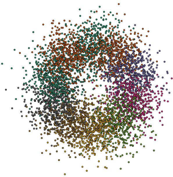
In this visualization, edges connect nodes based on color similarity. Same-color connections are “easy,” while connections between distant colors are “hard.”

The researchers then tracked which edges the model chose to mask over time.

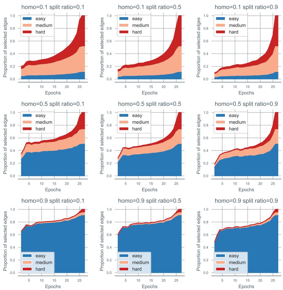
Look at the charts above. The Blue areas represent “Easy” edges, Orange are “Medium,” and Red are “Hard.”

• Early Epochs (Left side of x-axis): The selection is dominated by Blue (Easy).
• Later Epochs (Right side of x-axis): The Red (Hard) areas expand significantly.

This empirically proves that the self-paced scheduler works exactly as intended, autonomously discovering and ramping up difficulty.

4. Ablation Studies: Do we need all the parts?

Science requires verification. The authors stripped parts of the model to see what happened.

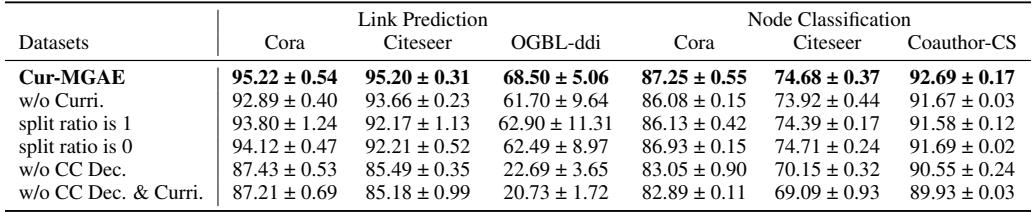
• w/o Curri: Removing the curriculum and using random masking dropped performance significantly.
• Split ratio is 1: Using only difficulty-based selection (no randomness) caused overfitting and lower results.
• w/o CC Dec: Replacing the Cross-correlation decoder with a simple dot product hurt performance drastically, showing the importance of the advanced decoder.

5. Parameter Sensitivity

How robust is the model to hyperparameter changes?

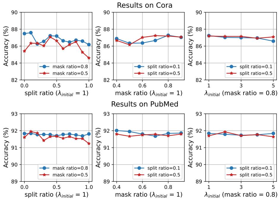
The charts show stable performance across reasonable ranges. The Split Ratio (left column) shows that a balance (around 0.5 to 0.8) is better than extremes (0 or 1), confirming the need for a mix of curriculum and randomness.

Theoretical Analysis: Why it Converges

One might worry that changing the training data (the mask) dynamically could make the training unstable. The authors provide a rigorous theoretical proof.

They analyze the convergence using the Hessian matrix (second-order derivatives).

By proving that the objective function is smooth and bounded (Lipschitz continuous gradient), they demonstrate that Algorithm 1 is guaranteed to converge to a stationary point. In simple terms: despite the moving target of the curriculum, the math guarantees the model will settle on a solution.

Conclusion

The Cur-MGAE paper highlights a fundamental truth in learning: the order of information matters. By moving away from random masking and embracing a structure-aware curriculum, the authors have created a Graph Autoencoder that learns more efficiently and effectively.

Key Takeaways:

1. Context Matters: Reconstructing edges isn’t just about presence/absence; it’s about difficulty relative to the remaining structure.
2. Start Simple: Masking easy edges first builds a foundation.
3. Mix it Up: A rigid curriculum leads to overfitting; mixing in random exploration keeps the model robust.

This work paves the way for smarter self-supervised learning, potentially allowing GNNs to tackle even larger and more complex networks in biology, social media, and physics without needing millions of human labels. Just like students, AI learns best when the syllabus is well-planned.