](https://deep-paper.org/en/paper/file-3083/images/cover.png)
Introduction
Imagine you are reading the following sentence:
“I eat an apple while holding my iPhone.”
As a human, your brain performs a lightning-fast calculation. You instantly understand that the word “apple” refers to the fruit, not the technology giant Apple Inc., even though the context contains the word “iPhone.” This ability to determine which meaning of a word is intended based on context is called Word Sense Disambiguation (WSD).
For a long time, WSD was a holy grail in Natural Language Processing (NLP). With the arrival of powerful pre-trained language models (LMs) like BERT and GPT, the community largely declared victory. These models, equipped with “contextualized embeddings,” seemed to handle these homonyms effortlessly, achieving near-human performance on standard benchmarks.
But a recent paper titled “FOOL ME IF YOU CAN!” poses a provocative question: Is the problem actually solved, or have we just been giving the models easy tests?
Researchers from the University of Osnabrück suggest that while models are great at pattern matching, they might lack true contextual understanding. To prove this, they created FOOL, a dataset designed to trick models using adversarial contexts. In this post, we will break down their methodology, explore how they “broke” state-of-the-art models, and analyze what this means for the future of AI robustness.
The Background: Homonyms and Context
To understand the paper, we first need to define the core linguistic challenge: Homonyms. These are words that share the same spelling and pronunciation but have completely unrelated meanings.
Common examples include:
- Bank: A financial institution vs. the side of a river.
- Bat: A nocturnal flying mammal vs. a piece of sports equipment.
- Crane: A bird vs. a construction machine.
In NLP, there are two ways to test a model’s ability to distinguish these meanings:
- Fine-grained WSD: Distinguishing subtle nuances (e.g., “bank” as a building vs. “bank” as the institution itself).
- Coarse-grained WSD: Distinguishing entirely different meanings (River vs. Money).
This research focuses on coarse-grained WSD. Logic dictates that this should be easy for modern AI. After all, if a model has read the entire internet, it should know that “feathers” usually relate to the bird “crane,” not the bulldozer. However, the researchers suspected that models rely too heavily on specific “trigger words” rather than understanding the full sentence structure.
The Core Method: Building the “FOOL” Dataset
The heart of this research is the construction of the dataset itself. The authors didn’t just want to test if a model knows what a “bat” is; they wanted to test if the model could hold onto that meaning when the rest of the sentence is trying to trick it.
They created a dataset covering 20 distinct homonyms, structured into four progressively difficult test sets.
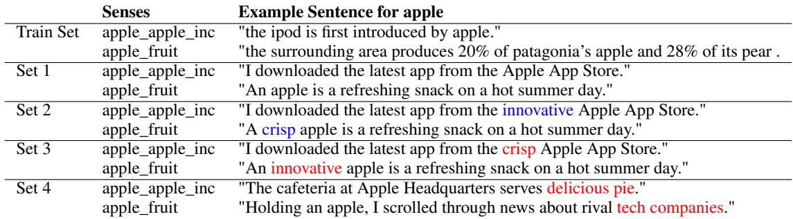
As shown in Table 1 above, the complexity ramps up significantly across the sets:
- Set 1 (Regular): The baseline. The homonym is used in a standard, anticipated context.
- Example: “The iPod is first introduced by apple.”
- Set 2 (Regular + Adjective): Similar to Set 1, but a supportive adjective is placed right before the target word.
- Example: “The surrounding area produces 20% of Patagonia’s apple…”
- Set 3 (Artificial Adversarial): This is where the “trap” is set. The authors take a sentence where the word means “Fruit,” but they insert an adjective typically associated with the “Company” meaning (or vice versa).
- Example: “An innovative apple is a refreshing snack…”
- Here, “innovative” screams “Apple Inc.” to a statistical model, but the syntax clearly describes a fruit.
- Set 4 (Realistic Adversarial): These are natural, realistic sentences that contain opposing context words.
- Example: “Holding an apple, I scrolled through news about rival tech companies.”
- This is the hardest test. The sentence talks about tech companies, but the physical act of “holding” implies the fruit.
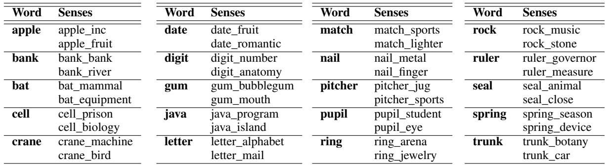
The researchers curated 20 homonyms to run through these gauntlets. You can see the full list of words and their dual meanings in Table 2 below.
Experiment 1: Probing the “Brain” of Encoder Models
The researchers tested two distinct families of AI models. The first group consists of Encoder models (like BERT and T5). These models process an entire sentence simultaneously (bidirectionally) and create a mathematical representation, or “embedding,” for every word.
To test these models, the researchers didn’t just ask them a question. They extracted the embedding vectors—the model’s internal thought representation—of the target word. They then used a k-Nearest Neighbor (kNN) algorithm to see if the embeddings for “Apple (Fruit)” clustered separately from “Apple (Company).”
If the model truly understands the difference, the mathematical representations should be far apart in vector space.
Visualizing the Failure
The results of this embedding analysis provided the most striking visual evidence in the paper. Using t-SNE (a technique to visualize high-dimensional data in 2D), the authors plotted how well the models separated the two meanings.
Take a look at Figure 1 below. The top row shows BERT-base, and the bottom row shows T5-base.
- Orange dots: Crane (Bird)
- Blue dots: Crane (Machine)
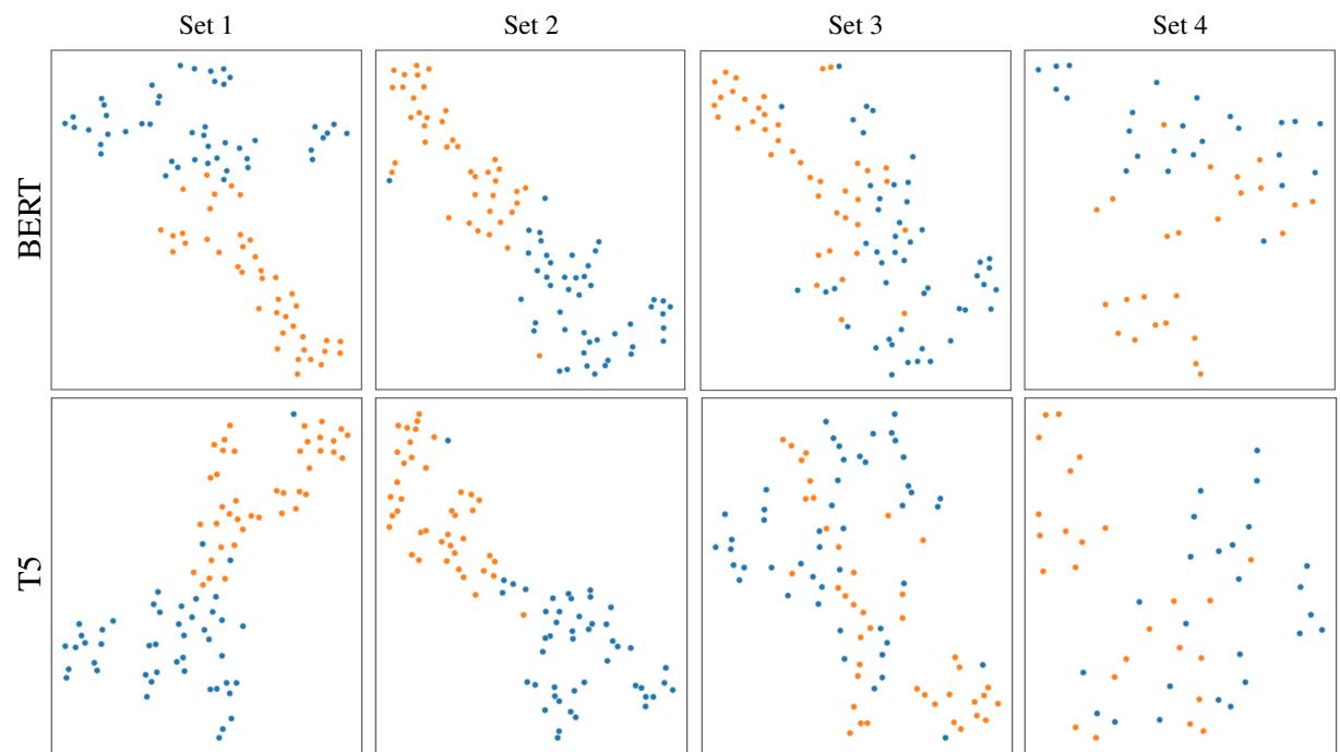
The breakdown is visible:
- Set 1 & 2: The blue and orange clusters are distinct. The models clearly distinguish the bird from the machine.
- Set 3: Look at the chaos. The clusters start to merge. The “adversarial adjective” is confusing the model’s internal representation.
- Set 4: In the realistic adversarial setting, the clusters are heavily overlapped. The model frequently cannot distinguish the senses based on its internal geometry.
Quantitative Results for Encoders
When we look at the raw accuracy numbers (F1-Scores), the trend confirms the visual data. Table 3 details the performance of various BERT and T5 models.
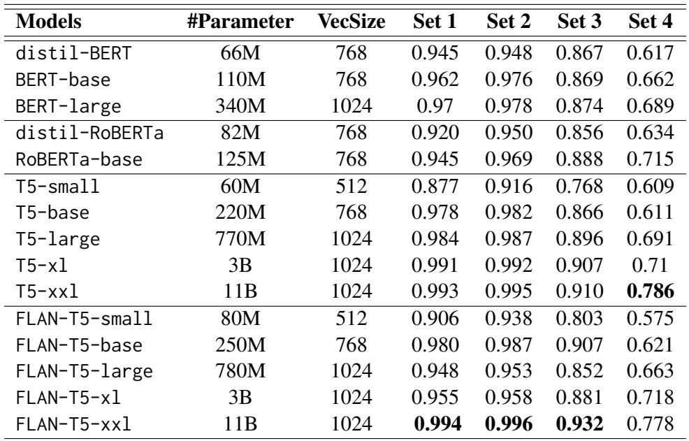
Key Takeaways from the Encoders:
- Sets 1 & 2 are easy: Almost every model scores above 95%.
- The “Set 4” Crash: Look at the drop-off. BERT-base goes from 96.2% accuracy on Set 1 down to 66.2% on Set 4.
- Size Matters: Larger models (like T5-xxl) are much more robust, maintaining a 78% score on Set 4. This suggests that simply adding more parameters helps the model resist being fooled, perhaps because it captures more nuanced context.
Experiment 2: Prompting Large Decoder Models (LLMs)
The second group of models tested were the Large Decoder Models, which include the heavy hitters like GPT-4, GPT-3.5 Turbo, and Llama 3. Since these models are designed to generate text, the researchers used Zero-Shot Prompting.
They essentially asked the model: “Classify the occurrence of the word ‘apple’ as fruit or company.”
Did the Giants Fall?
You might expect GPT-4 to ace this test. And largely, it did—but not without stumbling.
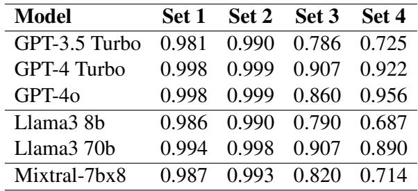
As shown in Table 4:
- GPT-4o is incredibly robust, scoring 95.6% even on the difficult Set 4.
- GPT-3.5 Turbo, however, struggles significantly. It drops from 98.1% (Set 1) to 72.5% (Set 4).
- Llama 3 (8b), a smaller open-source model, crashes to 68.7% on Set 4.
An Interesting Paradox: The researchers found a fascinating discrepancy. On Set 3 (where a misleading adjective is inserted, like “innovative apple”), some smaller encoder models (like BERT-large) actually outperformed massive decoder models.
- BERT-large (Set 3): 87.4%
- GPT-4o (Set 3): 86.0%
This suggests that bidirectional encoders (which see the whole sentence at once) might be slightly less susceptible to simple “distractor words” than autoregressive decoders (which read left-to-right), even if the decoders are much smarter overall.
Error Analysis: Where do models struggle?
Not all words are created equal. The researchers broke down the error rates by specific words to see if certain concepts were harder to disambiguate.
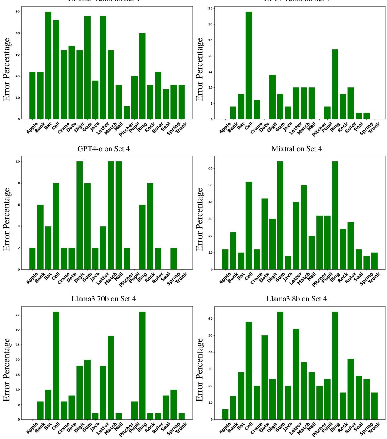
Looking at Figure 9 (above), which shows errors on the difficult Set 4, we see huge spikes for certain words:
- Digit: Models struggled massively to distinguish numbers from fingers/toes.
- Ring: Arena vs. Jewelry proved difficult in adversarial contexts.
Why these words? The authors suggest that words like “gum” (chewing gum vs. mouth gum) share very similar contexts (mouth, teeth, chewing), making them harder to separate than “Java” (Island vs. Code), which exist in entirely different semantic universes.
Conclusion and Implications
The “FOOL” paper serves as a necessary reality check for the AI industry. While we marvel at the generation capabilities of GPT-4 and Llama 3, this research highlights that robustness is not solved.
Key takeaways for students and researchers:
- Don’t trust benchmarks blindly: A model can score 99% on a standard test (Set 1) and fail miserably when a single adjective is changed (Set 3).
- Context is fragile: Models often rely on “trigger words” (like seeing “iPhone” and assuming “Apple Inc”) rather than parsing the grammatical relationship of the sentence.
- Architecture matters: Encoders (BERT/T5) and Decoders (GPT) fail in different ways. Encoders are surprisingly tough against simple adversarial adjectives, while massive Decoders are better at reasoning through complex, realistic scenarios.
The next time you use an LLM, remember: it might look like it understands you perfectly, but it might just be one “innovative adjective” away from total confusion.