When we think of Large Language Models (LLMs) like LLaMA or GPT-4, we usually think of them as masters of language. They write poetry, summarize emails, and debug code. But at their core, these models are sequence predictors—they look at a stream of tokens and predict what comes next.

This raises a fascinating question: If the sequence isn’t text, but data from a physical system, can the LLM learn the laws of physics just by looking at the numbers?

In a recent paper, researchers from Cornell University and Imperial College London explored this exact question. They discovered that LLMs can indeed “learn” the governing principles of dynamical systems—from chaotic weather models to stochastic stock market movements—without any fine-tuning. Even more impressively, they found that the models’ ability to understand these systems improves mathematically as they see more data, revealing a new kind of In-Context Neural Scaling Law.

In this post, we will tear down this research, explain the clever “Hierarchy-PDF” algorithm used to extract math from text models, and visualize how LLMs learn to simulate the world.

The Premise: From Text to Trajectories

To understand the magnitude of this study, we first need to define the problem. Dynamical systems are mathematical rules that describe how something changes over time. These can be:

1. Stochastic: Involving randomness (e.g., Brownian motion of particles).
2. Deterministic: No randomness, but potentially complex (e.g., the Lorenz system used in weather modeling).
3. Chaotic: Deterministic but highly sensitive to initial conditions.

The researchers wanted to know if a pre-trained LLM (specifically LLaMA-13b) could look at a sequence of numbers from these systems and figure out the underlying formula—the “transition rule”—purely from context.

The “Zero-Shot” Challenge

Usually, when we use machine learning for time series, we train a specific model on that data. Here, the researchers did not train the model. They simply fed a sequence of numbers (tokenized as text) into the LLM and asked it to predict the next state.

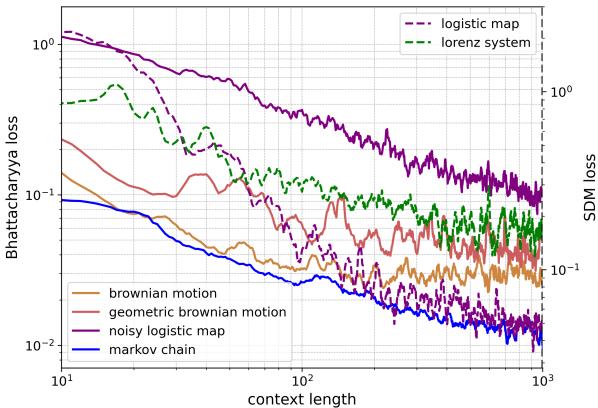
As shown in Figure 1 above, the results were striking. The graph shows the error rate (loss) dropping as the model sees more data (context length). Whether it’s the random walk of Brownian motion (solid orange) or the chaotic behavior of the Lorenz system (dashed green), the LLM gets better at predicting the physics as it reads more of the history.

The Methodology: Extracting Math from Language Models

How do you get a language model to output a precise probability distribution for a continuous number? An LLM outputs logits (scores) for tokens like “apple,” “code,” or “7.” It doesn’t naturally output a continuous probability density function (PDF).

To solve this, the authors developed a framework called Hierarchy-PDF.

1. Tokenizing the Physics

First, the time series data—which are floating-point numbers—must be converted into text. The researchers rescaled the data to a fixed interval and represented numbers as strings of digits. For example, a value might be represented as a 3-digit sequence.

The assumption is that the system follows a Markovian transition rule. This means the probability of the next state depends on the current state:

2. The Hierarchy-PDF Algorithm

This is the core innovation of the paper. Since the LLM predicts one token at a time, predicting a number like 5.23 is a hierarchical process.

1. Coarse Binning: The model predicts the first digit. If it assigns a high probability to the token “5”, it implies the value is likely between 5.0 and 6.0.
2. Refining: Given the first digit is 5, the model predicts the second digit. If it picks “2”, the range narrows to [5.20, 5.30].
3. Precision: This continues for the required number of digits.

This creates a tree structure. By querying the LLM for the probabilities of digits 0-9 at each level, the researchers can construct a highly detailed histogram that approximates the continuous probability distribution of the physics system.

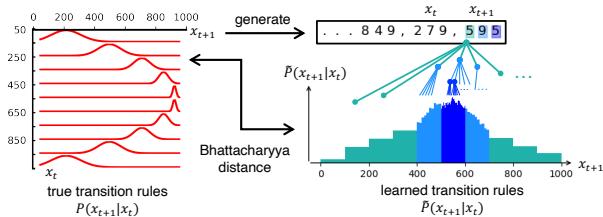
Figure 3 illustrates this beautifully. The “learned transition rules” (bottom right) are not just single point predictions. They are full probability distributions constructed by “zooming in” on the digits (color-coded by resolution). This allows the LLM to express uncertainty—a crucial feature for stochastic systems.

3. Discrete Systems

For simpler systems with discrete states (like a Markov chain that jumps between integers 0-9), the process is even more direct. The model just predicts the next token.

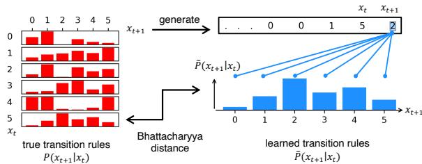
As seen in Figure 2, the researchers compare the “True” transition matrix (how the system actually works) with the “Learned” transition matrix derived from the LLM’s logits. They match surprisingly well.

4. Measuring Success: Bhattacharyya Distance

To quantify how well the LLM learned the physics, the researchers needed a metric to compare two probability distributions: the True distribution (derived from the math equations) and the Predicted distribution (extracted from the LLM).

They chose the Bhattacharyya distance.

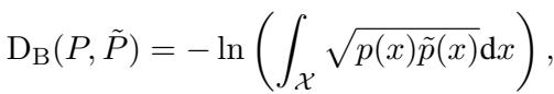
In simple terms, this measures the overlap between two statistical populations. If the LLM’s predicted “cloud” of probabilities overlaps perfectly with the reality of the physics equation, the distance is zero.

Experiments: The Zoo of Dynamical Systems

The researchers tested LLaMA-13b on a variety of systems to see if it was memorizing numbers or actually learning rules.

Case 1: Discrete Markov Chains

They started with a randomly generated Markov chain. This is a system where the next state is determined purely by probabilities defined in a matrix:

Because the matrix is random, the LLM cannot rely on pre-training knowledge. It must look at the context window to figure out the probabilities.

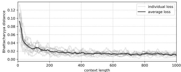
Figure 4 shows the result. The Bhattacharyya distance (error) collapses rapidly. With a context length of zero, the model knows nothing. But as it sees 100 or 200 steps of the chain, it reverse-engineers the random matrix that created the data.

Case 2: Stochastic Systems (Brownian Motion)

Next, they moved to continuous stochastic processes. The classic example is Brownian motion—the random movement of particles suspended in a fluid. This is governed by a stochastic differential equation:

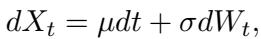
Here, \(dW_t\) represents the random “noise” or increments. The transition rule is a Gaussian (Normal) distribution.

The LLM was able to reconstruct this Gaussian shape perfectly.

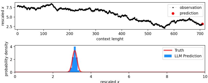
In Figure 10, the red line is the ground truth (a bell curve). The blue histogram is the LLM’s prediction. The model didn’t just guess the mean (the center); it correctly estimated the variance (the width) of the noise.

Case 3: Chaotic Systems (The Logistic Map)

Perhaps the most difficult test is Chaos. Chaotic systems are deterministic (no randomness) but extremely sensitive. A tiny change in the start leads to wildly different outcomes.

The researchers used the Logistic Map, a model for population growth:

When the parameter \(r=3.9\), this system behaves chaotically.

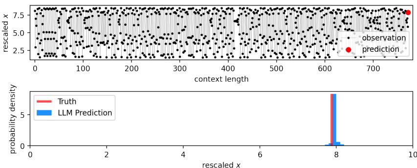
Look at Figure 15. The top plot shows the chaotic time series. The bottom plot shows the prediction for the last step.

• Truth (Red Line): Since the system is deterministic, the “true” probability is a spike (a Dirac delta function) at the exact correct value.
• Prediction (Blue Bar): The LLM places almost all its probability mass exactly on that value.

It has “solved” the equation just by looking at the sequence.

Learning the Noise in Chaos

The researchers then added noise to the Logistic Map to make it stochastic. Now the model has to predict a moving target with changing variance.

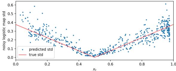
Figure 7 (bottom plot) is particularly impressive. The red line shows the true standard deviation (volatility) of the system, which changes depending on the current value \(x_t\). The blue dots are the LLM’s predicted standard deviation. The model learned that uncertainty isn’t constant—it varies depending on the state of the system.

The Discovery: An In-Context Neural Scaling Law

The most profound finding in this paper is not just that LLMs can learn these systems, but how they learn them.

In deep learning, we are familiar with “Scaling Laws”—empirical rules that say “if you double the model size or data size, the loss decreases by X amount.” These usually apply to training.

This paper proposes an In-Context Neural Scaling Law. It describes how the model’s understanding of the physical rules improves as the length of the prompt (context window) increases.

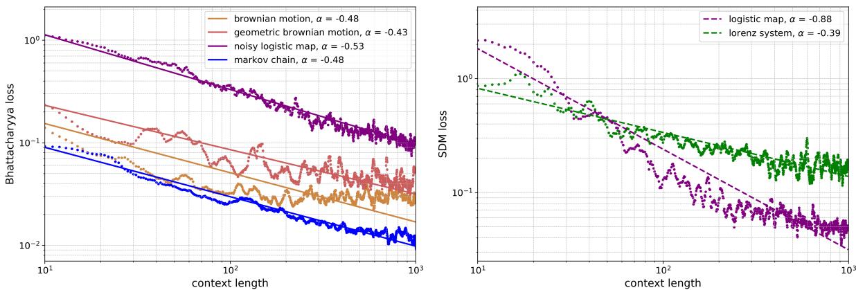
Figure 20 displays these power laws.

• Left (Stochastic): The straight lines on the log-log plot indicate a power-law relationship. For the “Noisy Logistic Map” (purple), the error drops consistently as the context length grows from 10 to 1,000.
• Right (Deterministic): The Logistic Map (magenta) shows a steep descent.

The equation governing this behavior is:

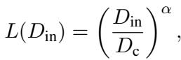
Where \(D_{in}\) is the context length and \(\alpha\) is the scaling exponent. This suggests that LLMs are performing a type of data-driven algorithm internally, similar to how a statistician would update their confidence intervals as they collect more samples.

Discussion: Is it just Memorization?

A skeptic might ask: “Is the LLM actually learning physics, or is it just matching patterns it saw in its massive training data?”

To test this, the authors compared the LLM against standard baselines:

1. Unigram/Bigram models: Simple statistical counters.
2. AR1 (Autoregressive) Models: Standard time-series tools.
3. Neural Networks: A small neural net trained specifically on the sequence in real-time.

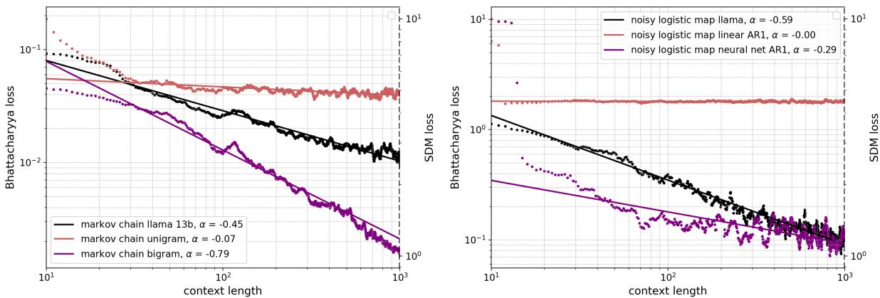
Figure 21 shows the comparison.

• Left (Markov Chain): The LLaMA model (black) performs comparably to the Bigram model (purple), which is the theoretical ideal for this task.
• Right (Noisy Logistic Map): The LLaMA model beats the linear AR1 baseline (red) and matches the performance of a dedicated Neural Network (purple) trained on the spot.

This indicates that the LLM is implementing a learning algorithm in-context that is as effective as training a specialized neural network from scratch using Gradient Descent.

Conclusion and Implications

This research bridges the gap between natural language processing and scientific modeling. It demonstrates that Large Language Models are not merely “stochastic parrots” repeating text; they are general-purpose pattern recognition engines capable of inferring complex mathematical rules.

The key takeaways are:

1. Zero-Shot Physics: LLMs can model stochastic, chaotic, and continuous systems without fine-tuning.
2. Hierarchy-PDF: We can extract precise, multi-resolution probability distributions from LLMs, allowing them to act as simulators.
3. In-Context Scaling: The accuracy of the learned physics scales with the context length following a power law, behaving like a legitimate statistical learning algorithm.

This opens the door to using LLMs for analyzing experimental data where the underlying equations are unknown. Instead of manually deriving a model, we might one day simply feed the data into an LLM and ask it to describe the laws of the universe.