Beyond the Final Layer—Extrapolating Emotion in LLMs

Introduction

Imagine you are texting a friend. They reply: “You can’t change who people are, but you can love them #sadly.”

How do you classify the emotion here? A standard sentiment analysis tool might see the word “love” and tag it as Joy, or see the hashtag and tag it as Sadness. But a human reader detects something more nuanced: a sense of resignation, a difficult acceptance of reality. The correct label is likely Pessimism.

Large Language Models (LLMs) like GPT-4 or T5 have become incredibly adept at understanding text, but they still struggle with this level of fine-grained emotional nuance. They often hallucinate or default to “safe” labels like “Neutral” when the answer requires reading between the lines.

In this post, we will deep dive into a fascinating paper titled “Linear Layer Extrapolation for Fine-Grained Emotion Classification.” The researchers propose a novel method to extract these nuanced emotions not by training a larger model, but by changing how we read the model’s internal states. They reinterpret a technique called Contrastive Decoding through the lens of geometry, treating the model’s layers as a trajectory and “extrapolating” the prediction into a theoretical future layer.

Background: The Layered “Brain” of a Transformer

To understand this paper, we first need to visualize how a Transformer model processes information.

When you feed a sentence into a model like BERT or T5, it passes through a stack of layers (e.g., 12, 24, or 48 layers).

1. Early Layers: These typically focus on surface-level features—syntax, grammar, and basic word associations.
2. Middle Layers: These start to construct context and meaning.
3. Late (Expert) Layers: These refine the understanding, handling complex reasoning, factuality, and nuance.

The Concept of Early Exiting

Usually, we only care about the output of the final layer. However, we can perform an “early exit.” This means we can take the internal state of the model at, say, Layer 15, attach a classifier to it, and ask: “What do you think the emotion is right now?”

Research shows that “factual” and “nuanced” abilities emerge in later layers. This led to the development of a technique called DoLa (Decoding by Contrasting Layers). The intuition is simple: if the Early Layer (the “Amateur”) thinks the text is just “Sad,” but the Final Layer (the “Expert”) thinks it is “Pessimistic,” we should emphasize the difference. We want to subtract the Amateur’s basic intuition to reveal the Expert’s nuanced insight.

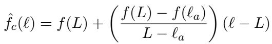
The Core Method: From Subtraction to Extrapolation

The authors of this paper take the concept of Contrastive Decoding and give it a rigorous mathematical and geometric foundation. They argue that we shouldn’t just subtract the amateur from the expert; we should view them as points on a line and extrapolate further.

1. The Standard Contrastive Approach

In standard Contrastive Decoding, we have two probability distributions:

1. \(p_e\): The Expert (Final layer) probabilities.
2. \(p_a\): The Amateur (Early layer) probabilities.

We want to boost the scores of classes where the Expert is much more confident than the Amateur. The standard formula looks like this:

Here, \(\beta\) is a hyperparameter that controls how much we penalize the amateur. If \(\beta\) is 0, we just use the expert. As \(\beta\) increases, we subtract more of the amateur’s score.

To ensure the model doesn’t go off the rails and pick a highly improbable word just because the amateur hated it, the authors use an Adaptive Plausibility Constraint. This filters the valid candidate classes (\(\mathcal{V}_{valid}\)) to include only those the expert considers somewhat likely:

Basically, we only perform this contrastive operation on the top-tier guesses from the expert.

2. Selecting the Amateur

Which early layer should be the “Amateur”? If you pick a layer too early (Layer 1), it knows nothing, so contrasting against it is useless. If you pick a layer too close to the end (Layer 47 out of 48), it’s identical to the expert, so the difference is zero.

The authors use a dynamic selection method. They compare the output distribution of the final layer against several early layers and pick the one that is most different (maximum distance).

This ensures the Amateur layer has a specific, distinct opinion that the Expert has since revised.

3. The Novel Insight: Linear Extrapolation

This is the most critical contribution of the paper. Instead of viewing the formula in Figure 2 as just “penalty subtraction,” the authors visualize it geometrically.

Imagine the model’s layers are steps on the x-axis. The model’s confidence in a specific emotion (the “logit score”) is on the y-axis.

• At Layer \(\ell_a\) (Amateur), the score for “Pessimism” is low.
• At Layer \(L\) (Expert), the score for “Pessimism” is higher.

If we draw a line through these two points, we can see a trajectory. The model is learning that the text is pessimistic as it gets deeper. Why stop at the final layer?

The authors propose projecting this line forward to a theoretical target layer \(\ell_t\) (e.g., Layer 60 in a 48-layer model). This is Linear Layer Extrapolation.

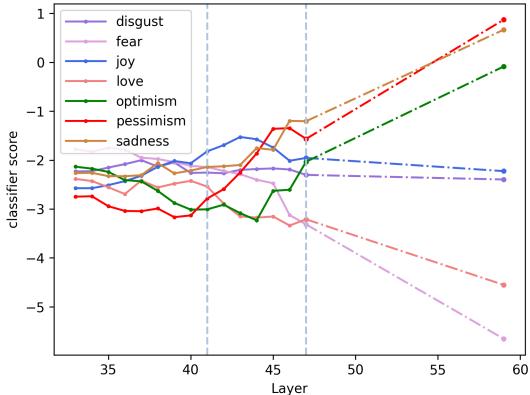
As shown in the image above, by extending the line past the final layer, the score for “Pessimism” (the dotted line) shoots up, eventually overtaking “Sadness.” This allows the model to correctly flip the prediction to the more nuanced class.

4. The Math of Extrapolation

Let’s formalize this. We have a line passing through the amateur score \(f(\ell_a)\) and the expert score \(f(L)\). The equation for a specific layer \(\ell\) on this line is:

The authors discovered that if you plug in the target layer \(\ell_t\) into this linear equation, it rearranges to look exactly like the standard Contrastive Decoding formula:

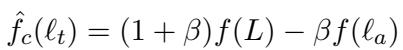
This is a powerful revelation. It means Contrastive Decoding is actually just Linear Extrapolation in disguise.

5. Dynamic Beta (\(\beta\)) Selection

In previous work, \(\beta\) (the contrastive strength) was a static number you had to guess (e.g., “let’s try 0.5”).

However, because the authors effectively linked \(\beta\) to the geometry of the layers, they can now define \(\beta\) dynamically. If the Amateur layer is far away from the Expert, the slope is different than if it is close.

The relationship between the target layer \(\ell_t\), the amateur layer \(\ell_a\), and \(\beta\) is:

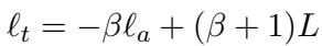
We can rearrange this to solve for \(\beta\):

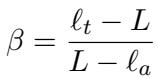
Why does this matter? Instead of blindly picking a fixed penalty \(\beta\), the researchers decide on a target layer (e.g., “I want to see what this model would look like if it had 10 more layers”). They set \(\ell_t\), and because the Amateur layer \(\ell_a\) changes dynamically for every input (based on which layer disagrees most with the expert), the \(\beta\) value automatically adjusts itself for every single sample.

This Dynamic \(\beta\) makes the method much more stable and robust.

Experiments and Results

The researchers tested this method on several challenging datasets, including goEmotions (28 fine-grained emotions), tweetEmotion, and tweetHate. They used FLAN-T5 and DeBERTa models.

Performance Gains

The results show a clear trend: Contrastive Classification outperforms standard classification, and the Dynamic \(\beta\) method generally yields the best results.

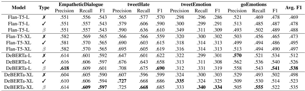
In Table 1, notice the Avg. F1 column on the far right. For almost every model (FLAN-T5, DeBERTa), the Dynamic \(\beta\) (marked with \(\beta\)) achieves the highest score compared to normal classification (\(\pmb{x}\)) or static beta (\(\checkmark\)).

The Effect of Extrapolating Further

How far into the “future” should we look? The authors experimented with setting the target layer \(\ell_t\) further and further out.

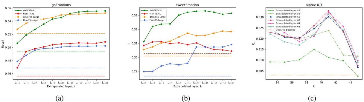
Looking at (a) in Figure 2, we see that for the goEmotions dataset, Recall improves as we extrapolate to higher layers (moving to the right on the x-axis). This confirms the hypothesis: the “direction” the model is moving in layer-by-layer is the correct one, and pushing further along that path refines the prediction.

Handling “Neutral” Bias

One of the biggest issues in emotion classification is that models love to play it safe. They often default to “Neutral” when the text is ambiguous.

The extrapolation method forces the model to be more opinionated. Because the “Neutral” probability usually stays flat or decreases across layers, while specific emotions (like “Curiosity” or “Disapproval”) rise, the extrapolation amplifies the specific emotion and suppresses the neutral one.

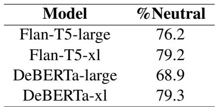
Table 2 highlights this success. For example, using DeBERTa-xl, nearly 80% of the samples that were flipped by this method were originally (and incorrectly) classified as Neutral.

Qualitative Examples

What does this look like in practice? The method successfully refines broad emotions into specific ones.

Table 3 shows common corrections. The models frequently moved from Sadness \(\rightarrow\) Pessimism or Joy \(\rightarrow\) Optimism. The model isn’t changing the sentiment polarity (positive/negative); it is refining the granularity.

We can see this evolution in the heatmaps of the model’s internal probabilities:

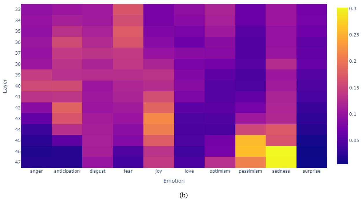
In the top example (a), notice how the probability for “Sadness” (the correct label in this specific context) starts low in the purple areas at early layers but brightens to yellow/orange in the later layers. A linear extrapolation takes this rising trend and projects it to a high confidence score, securing the correct prediction.

Stability of the Method

A major engineering benefit of the Dynamic \(\beta\) approach is stability. In standard contrastive decoding, you have to choose a hyperparameter \(k\) (the earliest layer to consider for the amateur). If you pick the wrong \(k\), performance crashes.

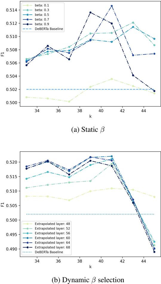
Figure 3 (top) shows that with a static \(\beta\), the F1 score fluctuates wildly depending on \(k\). However, Figure 3 (bottom) shows that with Dynamic \(\beta\), the performance (the colored lines) remains much more consistent regardless of which candidate layers are available. This makes the method much easier to deploy in real-world scenarios without endless hyperparameter tuning.

Conclusion

The paper “Linear Layer Extrapolation for Fine-Grained Emotion Classification” offers a compelling new way to think about how we extract information from Large Language Models.

The key takeaways are:

1. Layers as Trajectories: A model’s layers represent a journey from surface-level understanding to nuanced insight.
2. Extrapolation over Subtraction: Rather than just penalizing early mistakes, we should project the model’s internal evolution forward.
3. Dynamic Adaptation: By mathematically linking the contrastive penalty to the specific layers chosen, we can create a robust, adaptive decoding strategy.

This method requires no additional training—it simply gets more value out of the models we already have. It allows us to peel back the “Neutral” safety blanket models often hide under and reveal the subtle, fine-grained emotions that truly reflect human communication. As LLMs continue to integrate into social/emotional domains, techniques like Linear Layer Extrapolation will be essential for moving beyond robotic responses toward genuine empathy and understanding.